
Money Supply and Inflation after COVID-19


Department of Economics, Feliciano School of Business, Montclair State University, 1 Normal Avenue, Montclair, NJ 07043, USA
*
Author to whom correspondence should be addressed.
Economies 2022, 10(5), 101; https://doi.org/10.3390/economies10050101
Submission received: 22 March 2022
/
Revised: 25 April 2022
/
Accepted: 26 April 2022
/
Published: 28 April 2022
(This article belongs to the Special Issue International Financial Markets and Monetary Policy)
Abstract
:The core personal consumption expenditure (PCE) price index, the Federal Reserve’s preferred inflation gauge, rose to 5.2 percent on January 2022, which is the highest rate of increase since 40 years ago. Our estimates show that the annualized quarterly core PCE prices could reach 5.45% in the second quarter of 2022 and are as high as 8.57% in a longer time horizon unless corrected with restrictive monetary policies. Thus, the inflation shock since COVID-19 is not transitory, but it is persistent. As economists expect the Federal Reserve to tighten the money supply in March 2022, the insufficient policy responses may be attributed to a failure to incorporate a unique macroeconomic shock to unemployment during the pandemic. We propose a modified vector autoregression (VAR) model to examine structural shocks after COVID-19, and our proposed model performs well in forecasting future price levels in times of a pandemic.
Keywords:
inflation; forecast; time series; vector autoregressiion; pandemic; COVID-19; unemployment rate1. Introduction
“We tend to use [transitory] to mean that it won’t leave a permanent mark in the form of higher inflation. I think it’s probably a good time to retire that word and try to explain more clearly what we mean”, Federal Reserve Chairman Jerome Powell said during a congressional hearing on Tuesday, 2 December 2021.
To combat the negative economic effects of COVID-19, the Federal Reserve has used an unprecedented combination of monetary and fiscal policies. Clarida et al. (2021) provides an excellent summary of how the Federal Reserve deployed its conventional tools to support the U.S. economy in 2020 and contribute to robust economic recovery in 2021. The tools included large-scale asset purchase programs (Vissing-Jorgensen 2021), near-zero interest rates, and subsidized loan programs. On top of the expansionary monetary policies, Congress authorized various types of expansionary fiscal policies, including the $2.2 trillion Coronavirus Aid, Relief, and Economic Security (CARES) Act (Bhutta et al. 2020).
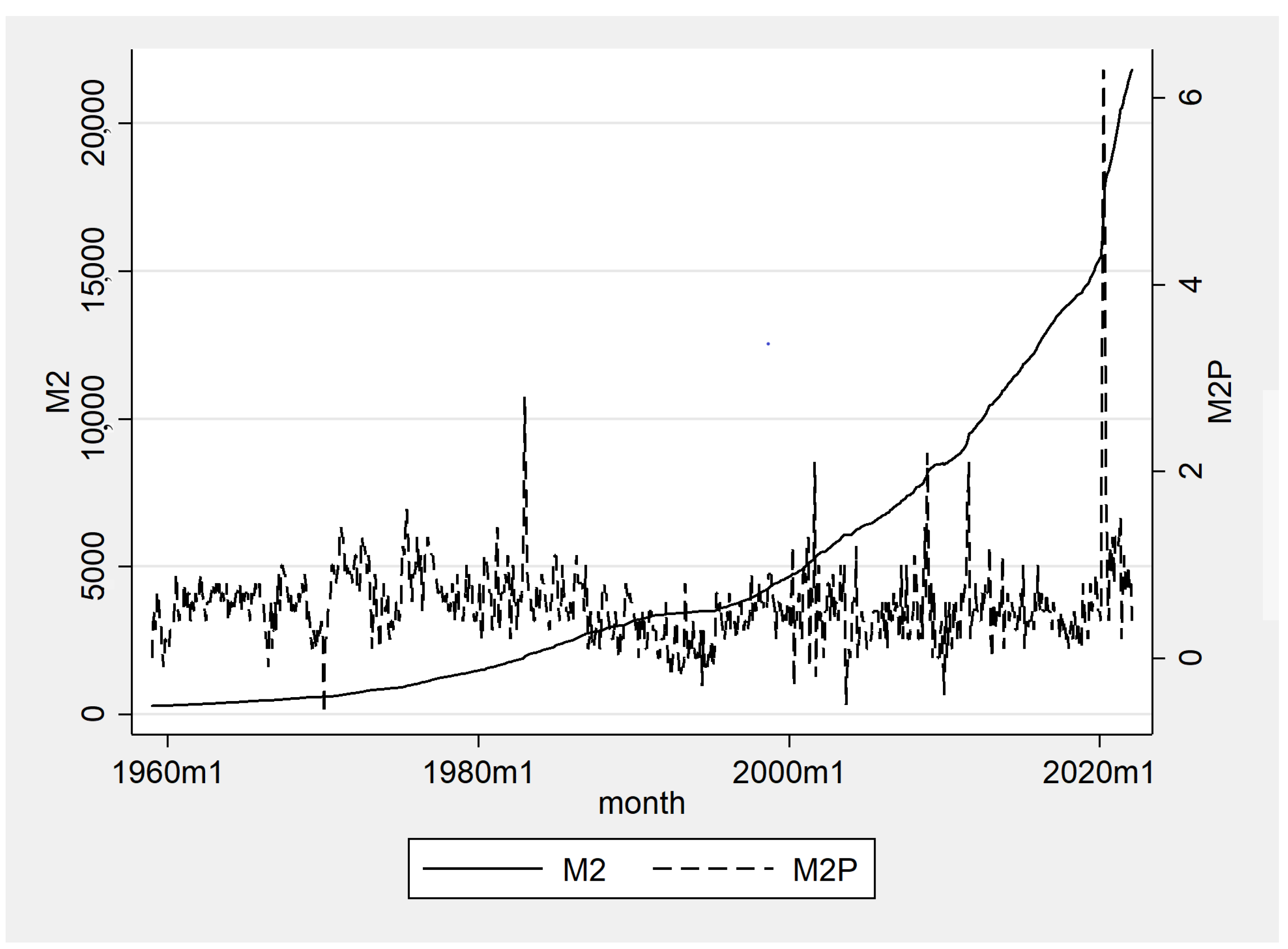
These expansionary monetary and fiscal policies led to a large increase in the supply of money. Figure 1 depicts M2 money supply (M2) in seasonally adjusted billions of dollars and its percent change (M2P) at a monthly level from 1959:01 to 2022:02. M2 since 1959 shows a slow and steady growth until 2000, growing to approximately $5 trillion in the 40-year span. Between 2000 and 2020, M2 grew from $5 trillion to $15 trillion, an increase of $10 trillion in 20 years. Due to the aforementioned expansionary policies in response to COVID-19, the level of M2 grew from approximately $15 trillion in 2020:01 to $22 trillion in 2022:02, an increase of $7 trillion in 2 years. The magnitude of the increase in M2 is quite astonishing compared to the rather slow and steady historical growth. At any month since 1959 and before 2020, the monthly percent change in M2 was within 2 percent except for 2.8 percent in 1983:01, which occurred during the oil shock crisis. Even during the Global Financial Crisis of 2007–2009, the monthly growth rate was within the 2 percent range. In contrast, the COVID-19 money supply growth rate is unprecedented. In March, April, and May 2020, the money supply grew by 3.4, 6.3, and 4.9 percent, respectively.
With the increase in the money supply, the debate about its impact on inflation has reemerged. The original idea behind the relationship between the money supply and inflation stems from the quantity theory of money (Humphrey 1974). The theory states that the quantity of money in circulation primarily affected the general level of prices. Brunner and Meltzer (1972); Brunner et al. (1980); Cagan (1989); Friedman (1989); Friedman and Schwartz (2008), and other monetarists show that a sudden increase in the money supply resulted in a proportional increase in inflation, and hence, the government should curtail the money supply to control the price level. In contrast, Ball et al. (1988); Cogley and Sbordone (2008); Del Negro et al. (2015); Galí (2015), and other Keynesian economists have challenged the quantity theory of money. The main argument is that an increase in the money supply has led to a decrease in the velocity of money and a rise in real income, which would stimulate aggregate demand and the economy would achieve full employment. For instance, Mishkin (2009) contends that the expansionary monetary policy was effective in reducing adverse effects from financial disruptions and managing an upward shift in inflation risks during the Global Financial Crisis.
However, the price level in the U.S. has substantially been increasing since 2021 and well into 2022. At the end of 2021, Federal Reserve Chairman Jerome Powell acknowledged that the upward trend in inflation is no longer transitory, reversing from the original stance.1 The headline U.S. inflation rate rose to 7.5 percent in January 2022, which is the highest rate of increase since 1982.2 The core personal consumption expenditure (PCE) price index, the Federal Reserve’s preferred inflation gauge, rose to 5.2 percent, also with the highest rate of increase since 1983.3 Given that the core PCE prices have been well over their target rate of 2 percent, the Federal Reserve increased the interest rate on March 2022, which is a major shift in the U.S. monetary policy, and it will continue to raise the rate at least until the end of 2022, although there is a disagreement about the incremental of each raise.4
Forecasting inflation after COVID-19 has been a difficult task using a traditional econometric model given the unique macroeconomic variations during the pandemic. Vector autoregression (VAR) is one of the most popular models in macroeconomics to measure the responses of outcome variables to exogenous shocks and forecast future outcomes (e.g., Giordano et al. 2007; Gharehgozli et al. 2020). However, the COVID-19 pandemic has created challenges to the VAR model, as the U.S. economy experienced economic disruptions at an unprecedented scale. Namely, the unemployment rate in April 2020 was 14.7 percent, an increase of 10 percentage points in a single month. Lenza and Primiceri (2020) point out that this type of unprecedented irregularity in the data will contaminate the pre-pandemic fit of the VAR model.
To tackle the challenge of using a VAR model in times of a pandemic, macro-econometricians are trying to incorporate this outlier, extreme observation, or contamination of data into the model. The literature provides two major solutions. A first strand of literature applies restrictions to the estimation. For instance, Lenza and Primiceri (2020) suggest an ad hoc strategy of removing outliers for parameter estimation. Economists can re-scale the April 2020 parameter, provided that this re-scaling is common to all shocks. The solution provides a flexibility in the model because the exact timing of the volatility change is known, which makes it much simpler than a typical time-varying volatility model. Unfortunately, the proposed solution is not suitable for forecasting because it significantly undermines uncertainty. Schorfheide and Song (2021) suggest that an existing mixed-frequency VAR model can still be used with some modification without a major ad hoc change. However, the modification still includes excluding a few months of outliers, which could jeopardize the model’s forecasting performance. A second strand of literature gets help from additional information. For instance, Foroni et al. (2020) use information from the Global Financial Crisis to adjust post-pandemic forecasts. Ng (2021) treats COVID-19 as a persistent health crisis with large economic consequences and “de-COVID” the data so that economic shocks within the VAR model can be identified. COVID-19 indicators, such as hospitalization, positive cases, and deaths, are used to either eliminate or include additional information for the modeling.
In line with the literature proposing alternatives to the traditional VAR approach, we propose a new model to examine the macroeconomic behaviors in times of a pandemic. Our model stems from the point of view that macroeconomic outcomes that originate with labor market dislocations differ from those in which labor markets play a less active role. Namely, domestic lockdown policies across different U.S. states in March and April 2020 served as an exogenous shock to unemployment. The domestic lockdown policies are unprecedented even in past epidemic episodes, which make the COVID-19 recession unique compared to any other historical crises. Furthermore, the so-called “Great Resignation”, during which workers have voluntarily decided not to return to work until work safety and an increase in real wages are guaranteed, has increased instability in unemployment. Thus, we assume that the labor market has been substantially distorted during the pandemic due to exogenous shocks, such as the lockdown policies and the Great Resignation. Our logic is in sync with an argument made in Aastveit et al. (2017), which show that the association between GDP and unemployment has been shifted since the Global Financial Crisis in 2008.
2. Model Specification
In this section, we introduce our VAR model and the identification scheme for the structural shocks and then discuss our data.
A VAR model is, in principle, a simple multivariate model in which each variable is explained by its own past values and the past values of all the other variables. In other words, it describes the evolution of a set of k variables, called endogenous variables, over time and, therefore, enables us to study the responses of each variable to substantial changes in others through the impulse response analysis, forecast error variance decomposition, historical decomposition, and the analysis of forecast scenarios (e.g., Hashimzade and Thornton 2021).
In the econometrics literature, the main stimulus for much recent work on VAR models is the paper by Sims (1980), based on the idea of using an unrestricted vector of past values of variables for forecasting. Since then, the literature has been full of studies in which a VAR is employed to study the relationship between economic indicators, and many of these studies are focused on the dynamics of the macroeconomic variables and the effects of events and interventions on these dynamics (e.g., Adeniran et al. 2016; Berisha 2020; Okoro 2014; Ronit and Divya 2014; Zuhroh et al. 2018).
One advantage of the VAR model is that we can typically treat all variables as a priori endogenous. Thereby, they account for Sims (1980)’s critique that the exogeneity assumptions for some of the variables in simultaneous equations models are ad hoc and often not backed by fully developed theories (e.g., Hashimzade and Thornton 2021). A VAR model does not assume any direction for the relationships unless restricted. Restrictions, including the exogeneity of some of the variables, may be imposed on VAR models based on statistical procedures. Structural VAR analysis, then, attempts to investigate structural economic hypotheses with the help of VAR models. While in the structural VAR, variables can have contemporaneous effects on each other, in a reduced-form structural VAR, the contemporaneous effects are considered in the error term, and while no variable has a direct contemporaneous effect on other variables, the occurrence of one structural shock can potentially lead to the occurrence of shocks in all error terms, thus creating contemporaneous movement in all endogenous variables.
There are some caveats in working with the VAR models. The estimation of autoregressive models requires that the data be fully observed. With the existence of missing values, this is not possible, rendering it impossible to estimate the model (e.g., Bashir and Wei 2018), or large samples of observations involving time series variables that cover many years are needed to estimate the VAR model; these are seldom available for regional studies (e.g., LeSage and Krivelyova 1999). VAR models are criticized because they do not shed any light on the underlying structure of the economy, as they do not aim to estimate causal relationships. Though this criticism is not important when the purpose of VAR is forecasting, it is relevant when the objective is to find causal relations among the macroeconomic variables.
We find that the structural VAR explained below is an appropriate model to address the inquiry of this study, which is not necessary to estimate the causal relationships between the variables in the model, but to employ their dynamics to forecast the future of the main variable of interest. The structural VAR enables us to follow and include the observed structural pattern of the economy (after the pandemic) and restrict the order of the shocks in the system to observe the responses of the variables.
2.1. Methodology
Nakamura and Steinsson (2018) provide a perspective on different identification strategies and approaches used to study the effect of monetary policy on macroeconomic indicators and describe their caveats. They give a critical assessment of several of the main methods, such as “matching moments”; those focused on identifying causal effects such as instrumental variables, difference-indifference analysis, regression discontinuities, randomized controlled trials; as well as vector autoregression. One important point they explain is the importance of finding an exogenous or surprise component of a monetary policy to assess the effects (and any “direct causal inference”). Romer and Romer (2004) suggest that the dispersion between realized values and the expected values of the indicators are the exogenous or unexpected component. Nakamura and Steinsson (2018) also discuss a standard VAR model regarding monetary policies and argue that an assumption must be made about whether the contemporaneous correlation between the variables is taken to reflect a causal influence. For instance, it is common to assume that the federal funds rate does not affect output and inflation contemporaneously.
VAR models are flexible multivariate time series models, which provide a rich account of the complex forms of autocorrelation and cross-correlation that are typical of macroeconomic variables. Bańbura et al. (2015); Del Negro et al. (2020); Giannone et al. (2015); Lenza and Primiceri (2020); Ng (2021); Romer and Romer (2004) all have different orderings of variables within the VAR model. In a typical VAR model, we can treat all variables as a priori endogenous. A VAR model does not assume any direction for the relationships, but restrictions, including the exogeneity of some of the variables, may be imposed based on statistical procedures. Structural VAR analysis, then, attempts to impose and investigate whether structural economic hypotheses and variables can have contemporaneous effects on each other. In a reduced-form structural VAR, the contemporaneous effects are considered in the error term, and the occurrence of one structural shock can potentially lead to the occurrence of shocks in all error terms, thus creating contemporaneous movement in all endogenous variables.
Consider the set of ; in our reduced-form VAR model, we perform:
is the intercept, and is the time trend; represents a 5 matrix collecting the estimated coefficients, and is the idiosyncratic error term. We discuss the choice of the variables further below, but the contribution of our model is the choice of the variables and the direction of the shocks, which the VAR model as described enables us to study. The pandemic and lockdowns caused an exogenous (dramatic) unemployment shock, followed by a severe shock in the economic activity (GDP). The supply of money was raised to a historical peak, and the velocity of money followed. This has caused contemporaneous and long-term effects on core inflation. Note that a VAR model does not assume any direction for the relationships. Therefore, the coefficients pick up the dynamics of the variables over the period under study without any arbitrary restriction put on any variables. Therefore, again, this model is first estimated without any restrictions.
Only in the case of the structural shocks, are identified from a Cholesky scheme restriction imposed on B such that or:
The variables of interest in our model are: real GDP per capita (GDPPC), measured in chained 2012 USD; unemployment rate (UNEMP), measured as the number of unemployed as a percentage of the labor force; M2 money supply (M2); velocity of money M2 (M2V); and core inflation (PCECORE), measured as personal consumption expenditures excluding food and energy (chain-type price index), as a percentage change from a year ago. All of our variables are seasonally adjusted and observed at a quarterly level. For a detailed explanation of the data sources and descriptions, please see Appendix A.
Note that the VAR model will capture the co-movement of the variables over time. However, we can set a scheme for the structural shocks. The contribution of our study is the choice of the direction of the shocks, which the VAR model as described above enables us to study. By design, the first structural shock stands for an exogenous (dramatic) unemployment shock caused by the pandemic and lockdowns, and stands for an output shock. Note that the order of the restrictions in this analysis is specific to the current pandemic and the economic responses. By nature, monetary and fiscal policies are high-dimensional, and over the time under study, other macroeconomics indicators were affected as well. We ordered the variables from the most to least exogenous based on our theory. The dramatic shock in the unemployment rate was indeed exogenous, caused by the severe lockdowns starting in March and April 2020. can be assumed to contemporaneously correspond to the unemployment shock and, along with the unemployment shock, to have contemporaneous effects on monetary policies and the supply of money. and refer to the shocks to money supply and velocity of money, which contemporaneously affect core inflation. Finally, refers to the shock to core inflation.
The main difference between the traditional VAR ordering and our VAR ordering is that we prioritized the exogenous shocks to the unemployment rate during the COVID-19 crisis. In previous recessions, such as during the Global Financial Crisis in 2008, a negative economic shock had a detrimental effect on GDP growth first. Then, the depressed economy caused an increase in the unemployment rate as the economy adjusted to the negative demand shock via employment. In contrast, we emphasize that macroeconomic variations after COVID-19 must be reorganized. U.S. states enforced unprecedented lockdown policies in March and April 2020, which had a direct impact on the labor market. Thus, this shock to the workforce was the most significant contributor to the inception and intensification of the COVID-19 recession. Our ordering of variables in the VAR model can best reflect the simultaneous effects of our variables of interest during the pandemic.
In our reduced-form structural VAR model, we estimate all the parameters from ordinary least squares (OLS) regressions. The Akaike information criterion (AIC) recommends the number of lags to consider in our model to be five. All series were seasonally adjusted, and we considered a constant and a trend in our series.
2.2. Data
We incorporated major macroeconomic indicators of the inflation suggested by the literature to understand the future direction of core prices, while considering the logical direction of the endogeneity of these indicators under the recent shocks caused by the pandemic. Then, we used a multivariate VAR model, which captures the historical dynamics of these major macroeconomic indicators of inflation and informs us about the future movements of these variables under current circumstances. We worked with the quarterly data of the unemployment rate, real GDP per capita, M2 money supply, the velocity of money, and core PCE prices. Our VAR model will provide the responses of these variables to the current shocks. The highly continuous co-variation of these series over a long period, incorporated in a VAR model that captures such variation of economic time series (without assuming any direction for causal relationship), enhances our ability to more precisely estimate and measure the magnitude of the shocks these series have encountered recently.
We used high-frequency data, observed at a quarterly level, over a long time series (1960:Q1 to 2021:Q4). The prediction of the dynamics of macroeconomic indicators at a higher frequency, especially for inflation, will help policymakers design appropriate monetary policies to circumvent the wide-ranging negative effects of the recession. The higher-frequency provides more degrees of freedom, which allows us to be more precise in understanding the relationship between inflation and the other indicators that directly affect core prices under the recent economic downturn.
As mentioned earlier, variables included in the analysis are real GDP per capita, the unemployment rate, M2 money supply, the velocity of money M2, and core inflation (for a detailed explanation of the data sources and descriptions, please see Appendix A).
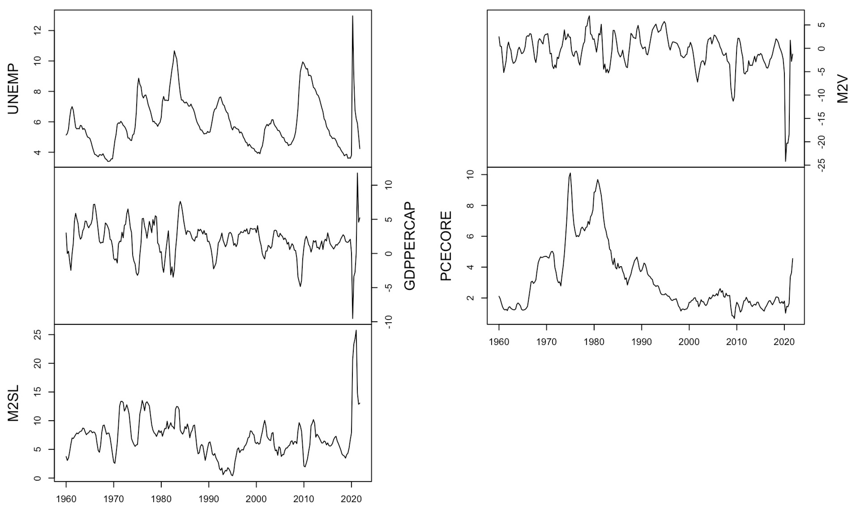
Figure 2 shows the time series of GDP per capita, the unemployment rate, M2, the velocity of money, and core inflation during the sample period from 1960:Q1 to 2021:Q4. Overall, the indirect relationship between GDP and the unemployment rate, as well as money supply and the velocity of money, is evident. However, the core inflation does not follow any clear pattern. In the early 1990s, the inflation rate was at around 4%, followed by a decline to 2% until late 1999. With the beginning of the year 2000, the inflation rate in the U.S. rose again, and it reached a peak in late 2007, which is officially known as the year when the U.S. economy slowed down and entered the Great Recession. With the beginning of the crisis, inflation followed the decline and stayed below 2% until the end of the sample period. Exceptions are the years 2011 and 2012, where the inflation rate in the U.S. was at around 3%. The recent shocks in these monetary indicators had never been experienced in the last six decades in the U.S. We provide a sensitivity analysis for the period of the Great Recession (2008:Q1 to 2009:Q2), but we should emphasize that the magnitude of the shocks are not comparable to that period.
3. Estimation Results
3.1. Main Results
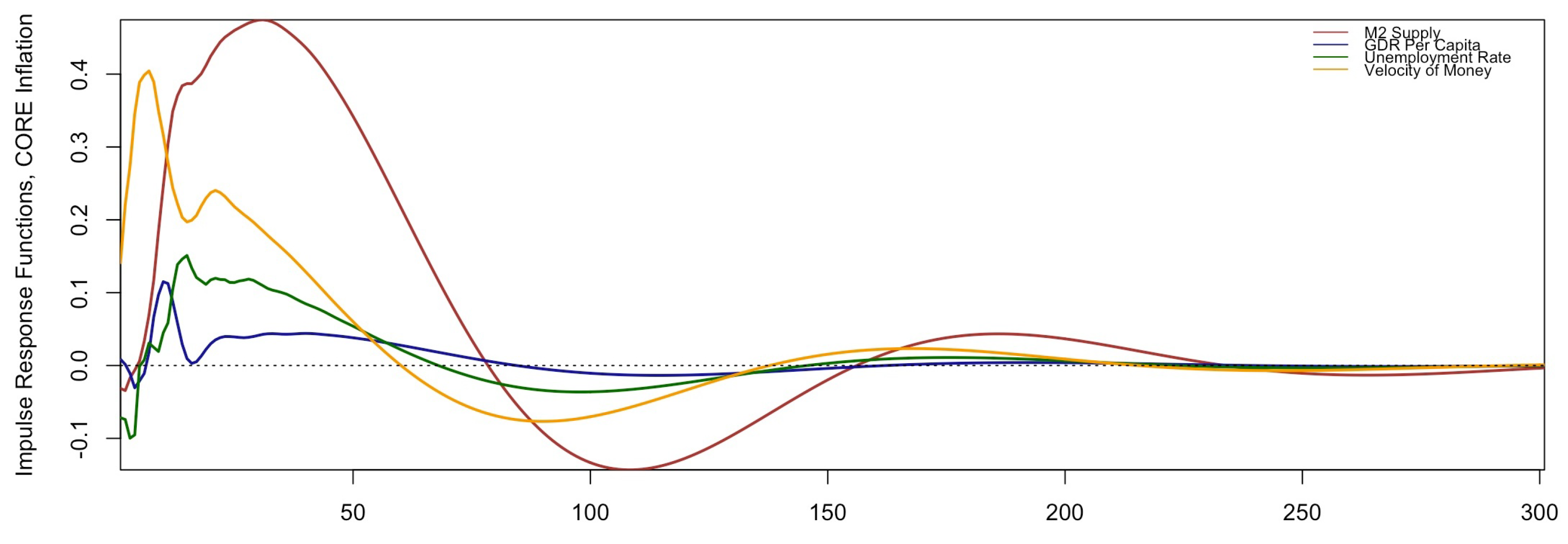
Figure 3 summarizes the impulse response functions (IRFs) of the main variables of interest, core inflation, to a one standard deviation positive shock in other indicators: unemployment rate, GDP per capita, M2, and velocity of money. By design, the most significant contemporaneous response is with respect to the velocity of money. A one standard deviation positive shock in the velocity of money significantly increases core inflation. Positive shocks in M2 have a lagged positive effect on core inflation. On the other hand, in the case of recessions when there is a negative shock in the unemployment rate, following the logical trend, core inflation shows a negative downward response. Note that we worked with real GDP per capita, while the velocity of money incorporates nominal GDP.
One standard deviation of the velocity of money (3.97 percent) would cause a maximum of a 0.404 percent increase in core inflation. The second quarter of 2020 recorded the highest negative shock in the velocity of money, with 6.1-times the standard deviation. This means that a potential positive response would amount to percent. One standard deviation of M2 (3.55 percent) would cause a maximum of a 0.475 percent increase in core inflation. The first quarter of 2021 recorded the highest positive shock in M2 with 7.27-times the standard deviation. This means that a potential positive response would amount to percent. Our findings suggest that, although the directions of the velocity of money and M2 shocks are opposite (as in Figure 2), even with the continuous increase in the money supply and with a recovering GDP, we expect a significant and persistent rise in core inflation during the COVID-19 crisis.
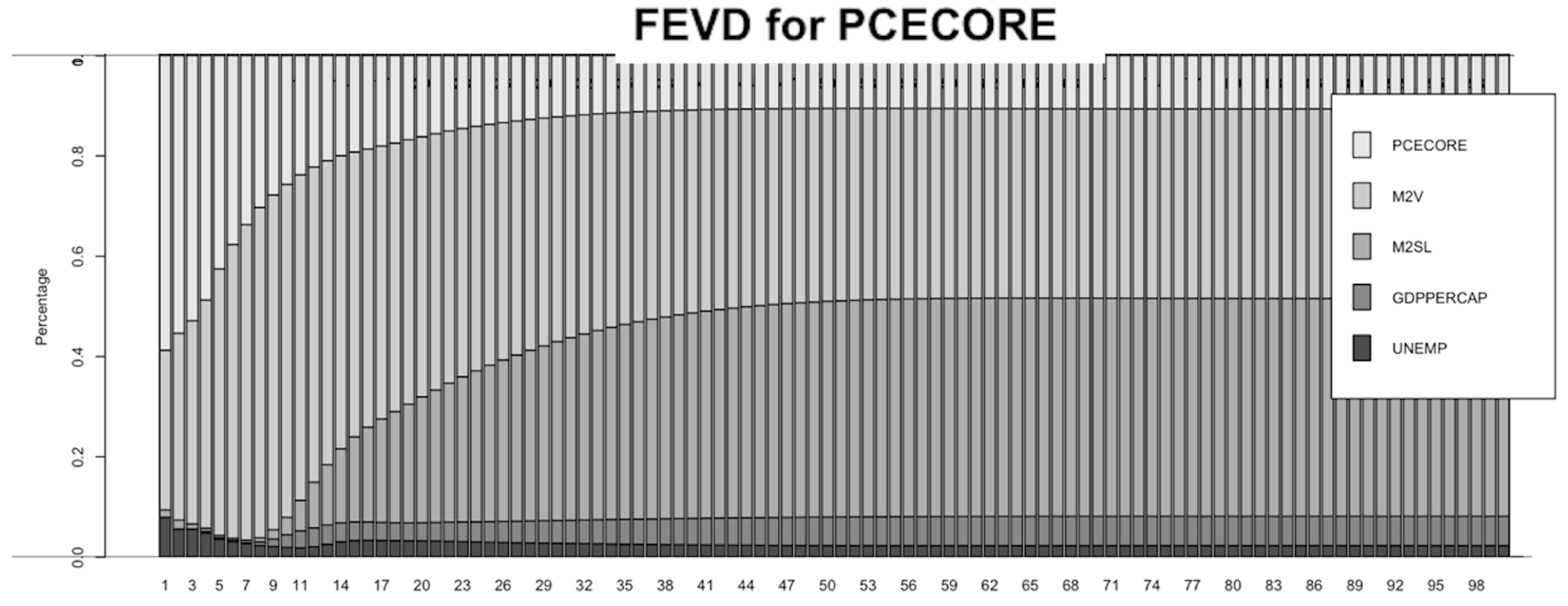
Figure 4 shows the forecast error variance decomposition (FEVD) for core inflation. The FEVD graph depicts the contribution of each individual shock as a share of the total area in a given time period. In the first quarter, we see that M2V, M2 money supply (M2SL), GDPPC, and UNEMP explain over 40 percent of the variability in core inflation, with M2V being the most significant explanatory indicator. M2V continues to play a substantial role in explaining variations in core inflation up to the ninth quarter. Beginning in the ninth quarter, we see an increasing role of M2 money supply (M2SL) as a component of the core inflation indicator, and the rising trend continues for several quarters onward. The decomposition analysis suggests that the substantial share of variations in core inflation can be explained initially by the velocity of money, then by the money supply. The result of the Granger test (order three) confirms the significance of the money supply indicator in defining core inflation with an F-statistic of 5.32 and p-value of 0.001, while for the reverse relationship, the F-statistic is 1.66 with a p-value of 0.176, indicating an insignificant relationship.
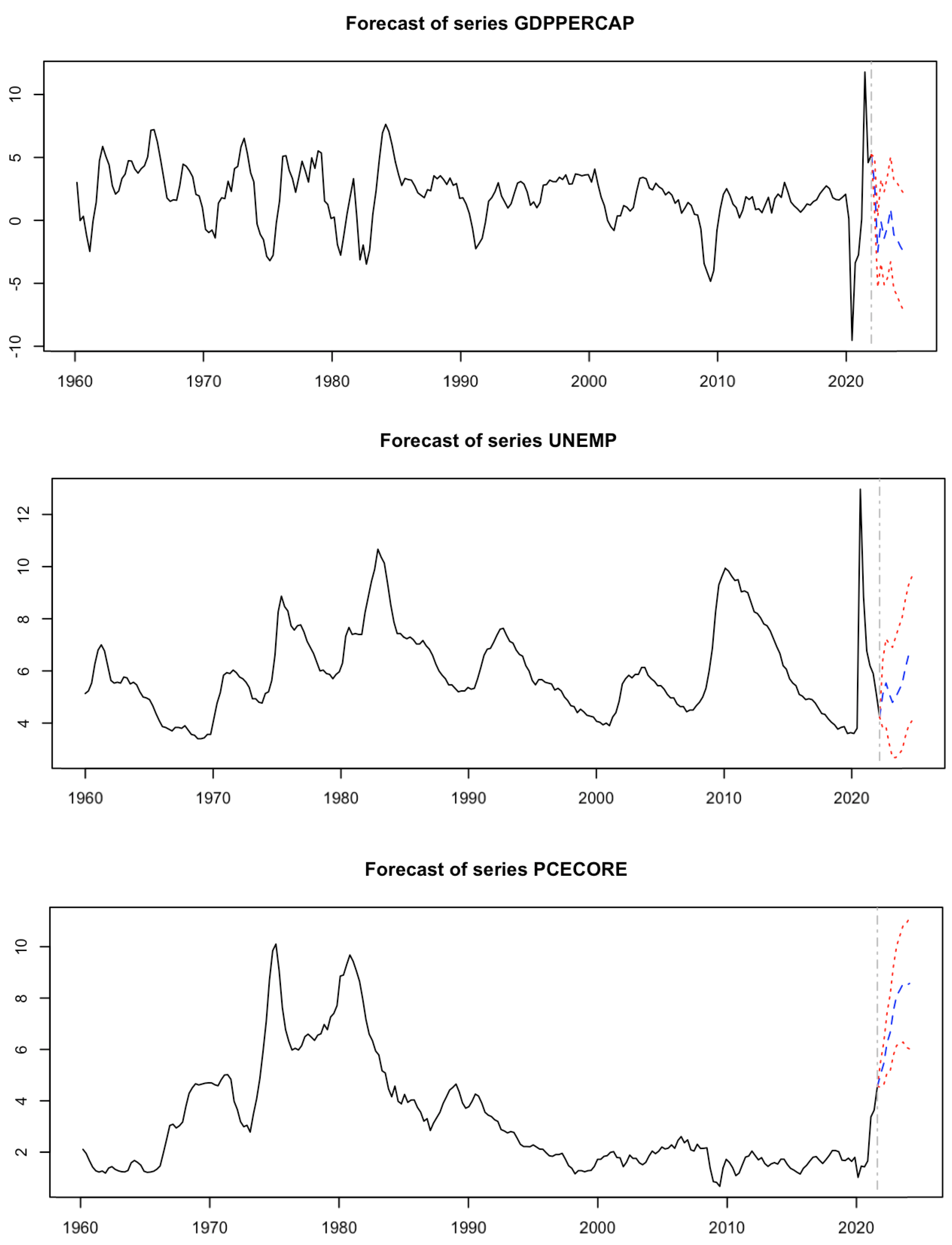
Assuming that M2V and M2 will have discretionary trends, Figure 5 shows the VAR forecast results for GDP per capita (GDPPC), the unemployment rate (UNEMP), and core inflation (PCECORE). The dashed vertical line represents the end of 2021. Hence, we are forecasting for the first quarter of 2022 and onward. Our model suggests that the unemployment rate will increase over 6 percent with a 95% confidence interval (CI). Adjustments in the labor market will continue during the first few quarters of 2022, as more people will be willing to work and actively seek employment. A gradual easement in COVID-19 health mandates in major states, such as New York relaxing mask mandates, will help contribute to an increase in the labor force. However, as more people return to the labor force, not all the newly added labor force will be able to secure employment. This is because we could experience a labor market surplus as firms may be reluctant to hire more workers at higher wages since the pandemic. As the labor market adjusts and the unemployment rate increases, our model suggests that our quarterly economic growth rate may decrease by approximately 2.5 percent.
Our estimates also indicate that core inflation will increase in the near future. For the first quarter of 2022, core inflation will rise to an average value of 5.03% (with a 95% CI of [4.53, 5.52]). For the second quarter of 2022, our model suggests that core inflation could increase to 5.45% (with a 95% CI of [4.62, 6.28]). Our forecasting analysis shows that inflation could rise as high as 8.57% (with a 95% CI of [6.02, 11.12]) in the future horizon. All of this evidence signals that the rise in inflation in the U.S. since 2021 is not “transitory”, but it is relatively “persistent”. Hence, the expansionary fiscal and monetary policies in 2020 will have a lingering effect on the U.S. economy unless corrected with contractionary policies.
3.2. Sensitivity Analysis
Our model assumes that the disruption to the labor market during the pandemic due to stringent lockdown policies resulted in an extreme unemployment rate of 14.7 percent in April 2020. No historical lockdown policies are comparable to that of the COVID-19 crisis, which makes the pandemic period VAR analysis unique. Aastveit et al. (2017) show that the evolution of the unemployment rate during the Global Financial Crisis is different relative to its past behavior. Even though the Global Financial Crisis and COVID-19 crisis are vastly different in terms of the underlying causes, economic consequences, and policy responses, these crises share a fundamental parameter instability in the unemployment rate. Thus, we examined whether our model can provide a robust forecasting estimate of inflation during the Global Financial Crisis in 2008.5
We restricted our sample period from 1690:Q1 to 2009:Q3 and introduced the Global Financial Crisis shocks accordingly. Then, we forecast core inflation from 2009:Q4 to 2010:Q4. Table 1 provides the values for actual inflation, predicted inflation using our VAR model, and the absolute difference between the two parameters, which we call dispersion. We see an absolute difference of 0.3 percentage points for the first quarter. In contrast, the subsequent dispersion values are very minimal, with a maximum difference of 0.1 percentage points. Thus, the sensitivity analysis result suggests that our VAR model specification is adequate for forecasting inflation, during which there is an idiosyncratic movement in unemployment.
4. Discussion
At the inception of our paper in mid-2021, the interest rate remained low and the Federal Reserve was cautious about raising the rates based on the “transitory” view of the rising inflation, as we discussed in Section 1. The unprecedented increase in the money supply as shown in Figure 1 and the uniqueness of the COVID-19 recession, especially with the domestic lockdowns in March and April 2020, as argued in Section 2.1, may have led to a more persistent upward shift in inflation. Our forecasts indicate that the core inflation rate will hover around a high 4% and the rate will continue to climb up in the near future. Hence, we have shown that a change in policy is necessary to correct for the upward pressure on the long-run inflation. In line with our prediction and given the persistent inflation, the Federal Reserve increased the interest rate on March 2022 by 0.25 percentage point6.
We compared our predictions in 2022 with other predictions and examined how our predictions fared against other forecasts. In a press conference on 16 March 20227, Federal Reserve Chairman Jerome Powell stated that the median inflation projection of FOMC participants is 4.3 percent in 2022, 2.7 percent in 2023, and 2.3 percent in 2024. Chairman Powell added that the recent trajectory is much higher than their own projection in December 2021 and noted that the FOMC participants continue to see risks as weighted to the upside. These estimates are similar to our predictions. Furthermore, a result from the monthly Bloomberg survey of 70 economists on April 2022 shows that the average core inflation for 2022 will be approximately 4.7%.8 Their estimate falls within our confidence interval.
The lockdowns in March and April 2020 and the consequent expansionary fiscal and monetary policies led to an unprecedented increase in the level of money supply. These government policies are not unusual as the Federal Reserve used conventional monetary tools such as lowering the interest rates and increasing asset purchases during the Global Financial Crisis (Mishkin 2009). However, the lesson from COVID-19 seems to indicate that forecasting inflation in times of a pandemic is different from in times of a financial crisis. The main difference was the lockdowns, which directly affected the unemployment rate, and our proposed model reflected this macroeconomic behavior. Hence, a major policy implication of our study is that the traditional ordering of the VAR model may not be sufficient when modeling the money supply and inflation in the current or future pandemics.
5. Conclusions
January 2022 marks the highest U.S. inflation rate in 40 years. The Federal Reserve began tightening the monetary policy in March 2022 to combat the high inflation. We showed that the traditional model of inflation forecasts may not capture all of the macroeconomic behaviors during a pandemic. The direct impact on the unemployment rate because of the lockdowns in March and April 2020 is the main difference from previous recessions. Incorporating this main difference into the model could have allowed us to realize that the COVID-19’s era inflation is not transitory.
Our proposed model predicts that the annualized quarterly core inflation rate could rise to 5.03% for the first quarter of 2022 and to 5.45% for the second quarter. In a longer time horizon, we forecast that the inflation rate could reach as high as 8.57% unless corrected with appropriate monetary policies. We also showed that the high inflation after COVID-19 is not transitory, but it is persistent. That is, the recent economic recovery and the excessive supply of M2 from fiscal and monetary policies have increased the core inflation rate beyond a transitory phase.
We contribute to the literature by proposing a changed VAR model specification to forecast inflation after COVID-19. The main modification is incorporating the exogenous shocks, namely domestic lockdown policies, to unemployment during the pandemic. Our proposed VAR model reflects the real macroeconomic behaviors during the pandemic, carefully contemplates the contemporaneous effects of these indicators, and performs well in forecasting future price levels. One of the main implications of our analysis is that the macroeconomic indicators during the recent pandemic-era recession may have different parameters than those from any other recessions. Failing to re-scale these differences may have contributed to the insufficient policy responses to the inflation shocks by the Federal Reserve.
We conclude with three caveats of our research. First, we designed our VAR strategy for forecasting inflation during a pandemic time only. Second, we did not incorporate inflation expectations. Third, our approach does not incorporate up-to-date methods, such as using high-frequency movement in interest rate futures around FOMC announcement dates or using external instrumental variables to identify monetary policy shocks. We believe these are important topics for future research.
Author Contributions
Conceptualization, O.G. and S.L.; Data curation, O.G. and S.L.; Formal analysis, O.G. and S.L.; Investigation, S.L.; Methodology, O.G. and S.L.; Writing—original draft, O.G.; Writing—review and editing, S.L. All authors have read and agreed to the published version of the manuscript.
Funding
This research received no external funding.
Conflicts of Interest
The authors declare no conflict of interest.
Appendix A
The data sources employed for the analysis are summarized in Table A1.

Table A1.
Descriptive statistics.
| Definition | Abbreviation Used | Source | |
|---|---|---|---|
| GDP Per Capita | Measured as real gross domestic product per capita, chained 2012 USD, Quarterly, seasonally adjusted, percent change from a year ago. | GDPPERCAP | U.S. Bureau of Economic Analysis, real gross domestic product per capita, retrieved from FRED, Federal Reserve Bank of St. Louis; https://fred.stlouisfed.org/series/A939RX0Q048SBEA, 1 February 2022. |
| Unemployment Rate | Represents the number of unemployed as a percentage of the labor force. Labor force data are restricted to people 16 years of age and older, who currently reside in 1 of the 50 states or the District of Columbia, and who are not on active duty. It is measured quarterly, and the data are seasonally adjusted. | UNEMP | U.S. Bureau of Labor Statistics, Unemployment Rate, retrieved from FRED, Federal Reserve Bank of St. Louis; https://fred.stlouisfed.org/series/UNRATE, 1 February 2022. |
| M2 Money Supply | Measured as percentage change from a year ago, seasonally adjusted quarterly data. | M2SL | Before May 2020, M2 consists of M1 plus (1) savings deposits (including money market deposit accounts); (2) small- denomination time deposits (time deposits in amounts of less than USD 100,000) less individual retirement account (IRA) and Keogh balances at depository institutions; and (3) balances in retail money market funds (MMFs) less IRA and Keogh balances at MMFs. Beginning May 2020, M2 consists of M1 plus (1) small-denomination time deposits (time deposits in amounts of less than USD 100,000) less IRA and Keogh balances at depository institutions; and (2) balances in retail MMFs less IRA and Keogh balances at MMFs. Seasonally adjusted M2 is constructed by summing savings deposits (before May 2020), small-denomination time deposits, and retail MMFs, each seasonally adjusted separately, and adding this result to seasonally adjusted M1. Board of Governors of the Federal Reserve System (U.S.), M2 Money Stock, retrieved from FRED, Federal Reserve Bank of St. Louis; https://fred.stlouisfed.org/series/M2SL, 1 February 2022. |
| Velocity of Money M2 | Measured as percentage change from a year ago, seasonally adjusted quarterly data. | M2V | Federal Reserve Bank of St. Louis, velocity of M2 Money Stock, retrieved from FRED, Federal Reserve Bank of St. Louis; https://fred.stlouisfed.org/series/M2V, 1 February 2022. |
| Inflation | Personal consumption expenditures excluding food and energy (chain-type price index), as percentage change from a year ago, seasonally adjusted quarterly data. | PCECORE | U.S. Bureau of Economic Analysis, Personal Consumption Expenditures: Chain-type Price Index, retrieved from FRED, Federal Reserve Bank of St. Louis; https://fred.stlouisfed.org/series/PCEPI, 1 February 2021. |
Table A2 provides the descriptive statistics.
Table A2.
Descriptive statistics.
| Mean | Std. Dev. | Min | Max | Median | |
|---|---|---|---|---|---|
| GDP Per Capita | 1.96 | 2.41 | −9.53 | 11.78 | 2.02 |
| Unemployment Rate | 5.99 | 1.66 | 3.40 | 12.97 | 5.70 |
| Money Supply M2 | 7.15 | 3.55 | 7.15 | 25.77 | 6.93 |
| Velocity of Money M2 | −0.66 | 3.97 | −24.19 | 6.95 | −0.34 |
| Core Inflation | 3.20 | 2.13 | 0.67 | 10.10 | 2.21 |
[custom] References
| 1 | Siegel, Rachel. 2021. “The Fed’s inflation challenge: Getting the policy and the messaging right”. Washington Post, December 9. https://www.washingtonpost.com/business/2021/12/09/inflation-fed-transitory-powell/ (accessed on 1 March 2022). |
| 2 | Politi, James, and Kate Duguid. 2022. “US inflation surges to 7.5% in fastest annual rise for 40 years”. Financial Times, February 10. https://www.ft.com/content/7a0213d2-ad59-485f-bcc9-fc0e10a11988 (accessed on 1 March 2022). |
| 3 | Smith, Colby. 2022. “Fed inflation gauge heats up, raising pressure on officials to tighten policy”. Financial Times, February 25. https://www.ft.com/content/5fe1d820-c88a-4dd1-aedf-3ab1db815c82 (accessed on 1 March 2022). |
| 4 | Federal Reserve. 2022. Minutes of the Federal Open Market Committee, 15–16 March 2022. |
| 5 | Note that the order of exogenous shocks in the Great Recession was different than the recent one. The VAR model captures coefficients of a system of equations in which each variable depends on the lagged values of itself and others. Therefore, the change of order will not change the forecast values. However, the potential IRFs would be sensitive to the order of restrictions one could consider. |
| 6 | See Note 4 above. |
| 7 | Federal Reserve. 2022. “Press Conference Transcript”. 16 March. https://www.federalreserve.gov/mediacenter/files/FOMCpresconf20220316.pdf (accessed on 1 March 2022). |
| 8 | Pickert, Reade, and Kyungjin Yoo. 2022. “Economists Boost Inflation Expectations in Worrying Sign for Fed”. Bloomberg, April 8. https://www.bloomberg.com/news/articles/2022-04-08/economists-boost-inflation-expectations-in-worrying-sign-for-fed (accessed on 1 March 2022). |
References
- Aastveit, Knut Are, Andrea Carriero, Todd E. Clark, and Massimiliano Marcellino. 2017. Have standard vars remained stable since the crisis? Journal of Applied Econometrics 32: 931–51. [Google Scholar] [CrossRef] [Green Version]
- Adeniran, Abraham Oluwapelumi, Muhyideen Iyiola Azeez, and John Abiodun Aremu. 2016. External debt and economic growth in nigeria: A vector auto-regression (var) approach. International Journal of Management and Commerce Innovations 4: 706–14. [Google Scholar]
- Ball, Laurence, N. Gregory Mankiw, David Romer, George A. Akerlof, Andrew Rose, Janet Yellen, and Christopher A. Sims. 1988. The new keynesian economics and the output-inflation trade-off. Brookings Papers on Economic Activity 1988: 1–82. [Google Scholar] [CrossRef] [Green Version]
- Bańbura, Marta, Domenico Giannone, and Michele Lenza. 2015. Conditional forecasts and scenario analysis with vector autoregressions for large cross-sections. International Journal of Forecasting 31: 739–56. [Google Scholar] [CrossRef] [Green Version]
- Bashir, Faraj, and Hua-Liang Wei. 2018. Handling missing data in multivariate time series using a vector autoregressive model-imputation (var-im) algorithm. Neurocomputing 276: 23–30. [Google Scholar] [CrossRef]
- Berisha, Edmond. 2020. Tax cuts and” middle-class” workers. Economic Analysis and Policy 65: 276–81. [Google Scholar] [CrossRef]
- Bhutta, Neil, Jacqueline Blair, Lisa Dettling, and Kevin Moore. 2020. COVID-19, the cares act, and families’financial security. National Tax Journal 73: 645–72. [Google Scholar] [CrossRef]
- Brunner, Karl, Alex Cukierman, and Allan H. Meltzer. 1980. Stagflation, persistent unemployment and the permanence of economic shocks. Journal of Monetary Economics 6: 467–92. [Google Scholar] [CrossRef]
- Brunner, Karl, and Allan H. Meltzer. 1972. Money, debt, and economic activity. Journal of Political Economy 80: 951–77. [Google Scholar] [CrossRef] [Green Version]
- Cagan, Phillip. 1989. Monetarism. In Money. Berlin: Springer, pp. 195–205. [Google Scholar]
- Clarida, Richard H., Burcu Duygan-Bump, and Chiara Scotti. 2021. The COVID-19 crisis and the federal reserve’s policy response. Finance and Economics Discussion Series, 2021–35. [Google Scholar] [CrossRef]
- Cogley, Timothy, and Argia M. Sbordone. 2008. Trend inflation, indexation, and inflation persistence in the new keynesian phillips curve. American Economic Review 98: 2101–26. [Google Scholar] [CrossRef] [Green Version]
- Del Negro, Marco, Marc P. Giannoni, and Frank Schorfheide. 2015. Inflation in the great recession and new keynesian models. American Economic Journal: Macroeconomics 7: 168–96. [Google Scholar] [CrossRef] [Green Version]
- Del Negro, Marco, Michele Lenza, Giorgio E. Primiceri, and Andrea Tambalotti. 2020. What’s up with the Phillips Curve? Technical Report. Cambridge: National Bureau of Economic Research. [Google Scholar]
- Foroni, Claudia, Massimiliano Marcellino, and Dalibor Stevanovic. 2020. Forecasting the COVID-19 recession and recovery: Lessons from the financial crisis. International Journal of Forecasting 38: 596–612. [Google Scholar] [CrossRef] [PubMed]
- Friedman, Milton. 1989. Quantity theory of money. In Money. Berlin: Springer, pp. 1–40. [Google Scholar]
- Friedman, Milton, and Anna Jacobson Schwartz. 2008. A Monetary History of the United States, 1867–1960. Princeton: Princeton University Press, vol. 14. [Google Scholar]
- Galí, Jordi. 2015. Monetary Policy, Inflation, and the Business Cycle: An Introduction to the New Keynesian Framework and Its Applications. Princeton: Princeton University Press. [Google Scholar]
- Gharehgozli, Orkideh, Peyman Nayebvali, Amir Gharehgozli, and Zaman Zamanian. 2020. Impact of COVID-19 on the economic output of the us outbreak’s epicenter. Economics of Disasters and Climate Change 4: 561–73. [Google Scholar] [CrossRef]
- Giannone, Domenico, Michele Lenza, and Giorgio E. Primiceri. 2015. Prior selection for vector autoregressions. Review of Economics and Statistics 97: 436–51. [Google Scholar] [CrossRef] [Green Version]
- Giordano, Raffaela, Sandro Momigliano, Stefano Neri, and Roberto Perotti. 2007. The effects of fiscal policy in italy: Evidence from a var model. European Journal of Political Economy 23: 707–33. [Google Scholar] [CrossRef]
- Hashimzade, Nigar, and Michael A. Thornton. 2021. Handbook of Research Methods and Applications in Empirical Microeconomics. Cheltenham: Edward Elgar Publishing. [Google Scholar]
- Humphrey, Thomas M. 1974. The quantity theory of money: Its historical evolution and role in policy debates. FRB Richmond Economic Review 60: 2–19. [Google Scholar]
- Lenza, Michele, and Giorgio E. Primiceri. 2020. How to Estimate a Var after March 2020. Technical Report. Cambridge: National Bureau of Economic Research. [Google Scholar]
- LeSage, James P., and Anna Krivelyova. 1999. A spatial prior for bayesian vector autoregressive models. Journal of Regional Science 39: 297–317. [Google Scholar] [CrossRef]
- Mishkin, Frederic S. 2009. Is monetary policy effective during financial crises? American Economic Review 99: 573–77. [Google Scholar] [CrossRef] [Green Version]
- Nakamura, Emi, and Jón Steinsson. 2018. Identification in macroeconomics. Journal of Economic Perspectives 32: 59–86. [Google Scholar] [CrossRef] [Green Version]
- Ng, Serena. 2021. Modeling Macroeconomic Variations after COVID-19. Technical Report. Cambridge: National Bureau of Economic Research. [Google Scholar]
- Okoro, Edesiri Godsday. 2014. Oil price volatility and economic growth in nigeria: A vector auto-regression (var) approach. Acta Universitatis Danubius. OEconomica 10: 70–82. [Google Scholar]
- Romer, Christina D., and David H. Romer. 2004. A new measure of monetary shocks: Derivation and implications. American Economic Review 94: 1055–84. [Google Scholar] [CrossRef] [Green Version]
- Ronit, Mukherji, and Pandey Divya. 2014. The relationship between the growth of exports and growth of gross domestic product of india. International Journal of Business and Economics Research 3: 135–39. [Google Scholar] [CrossRef] [Green Version]
- Schorfheide, Frank, and Dongho Song. 2021. Real-Time Forecasting with a (Standard) Mixed-Frequency var during a Pandemic. Technical Report. Cambridge: National Bureau of Economic Research. [Google Scholar]
- Sims, Christopher A. 1980. Macroeconomics and reality. Econometrica: Journal of the Econometric Society 48: 1–48. [Google Scholar] [CrossRef] [Green Version]
- Vissing-Jorgensen, Annette. 2021. The treasury market in spring 2020 and the response of the federal reserve. Journal of Monetary Economics 124: 19–47. [Google Scholar] [CrossRef]
- Zuhroh, Idah, Hendra Kusuma, and Syela Kurniawati. 2018. An approach of vector autoregression model for inflation analysis in indonesia. Journal of Economics, Business & Accountancy Ventura 20: 261–68. [Google Scholar]
Figure 1.
M2 money supply (M2, left, billions of dollars) and M2 money supply percent change (M2P, right, %), monthly, seasonally adjusted, 1959:01–2022:02, Source: Board of Governors of the U.S. Federal Reserve System.
Figure 1.
M2 money supply (M2, left, billions of dollars) and M2 money supply percent change (M2P, right, %), monthly, seasonally adjusted, 1959:01–2022:02, Source: Board of Governors of the U.S. Federal Reserve System.

Figure 2.
Unemployment rate, real GDP per capita, and M2 on the left panel and velocity of money and core inflation on the right panel for 1960:Q1 to 2021:Q4; data series are quarterly data and are seasonally adjusted.
Figure 2.
Unemployment rate, real GDP per capita, and M2 on the left panel and velocity of money and core inflation on the right panel for 1960:Q1 to 2021:Q4; data series are quarterly data and are seasonally adjusted.

Figure 3.
Impulse response functions, and core inflation with respect to a shock in other indicators.
Figure 3.
Impulse response functions, and core inflation with respect to a shock in other indicators.

Figure 4.
Forecast error variance decomposition for core inflation.

Figure 5.
VAR forecast trends for GDP per capita, unemployment rate, and core inflation.

Table 1.
Actual inflation, predicted inflation, and absolute dispersion during the Financial Crisis in 2008.
Table 1.
Actual inflation, predicted inflation, and absolute dispersion during the Financial Crisis in 2008.
| Actual Inflation | Predicted Inflation | Dispersion | |
|---|---|---|---|
| 2009 Q4 | 1.4 | 1.7 | 0.3 |
| 2010 Q1 | 1.7 | 1.7 | 0.0 |
| 2010 Q2 | 1.6 | 1.5 | 0.1 |
| 2010 Q3 | 1.4 | 1.3 | 0.1 |
| 2010 Q4 | 1.1 | 1.1 | 0.0 |
Publisher’s Note: MDPI stays neutral with regard to jurisdictional claims in published maps and institutional affiliations. |
© 2022 by the authors. Licensee MDPI, Basel, Switzerland. This article is an open access article distributed under the terms and conditions of the Creative Commons Attribution (CC BY) license (https://creativecommons.org/licenses/by/4.0/).
Share and Cite
MDPI and ACS Style
Gharehgozli, O.; Lee, S. Money Supply and Inflation after COVID-19. Economies 2022, 10, 101. https://doi.org/10.3390/economies10050101
AMA Style
Gharehgozli O, Lee S. Money Supply and Inflation after COVID-19. Economies. 2022; 10(5):101. https://doi.org/10.3390/economies10050101
Chicago/Turabian StyleGharehgozli, Orkideh, and Sunhyung Lee. 2022. "Money Supply and Inflation after COVID-19" Economies 10, no. 5: 101. https://doi.org/10.3390/economies10050101
Note that from the first issue of 2016, this journal uses article numbers instead of page numbers. See further details here.