Nonlinear Combinational Dynamic Transmission Rate Model and Its Application in Global COVID-19 Epidemic Prediction and Analysis

Abstract

The outbreak of coronavirus disease 2019 (COVID-19) has caused a global disaster, seriously endangering human health and the stability of social order. The purpose of this study is to construct a nonlinear combinational dynamic transmission rate model with automatic selection based on forecasting effective measure (FEM) and support vector regression (SVR) to overcome the shortcomings of the difficulty in accurately estimating the basic infection number $R_0$ and the low accuracy of single model predictions. We apply the model to analyze and predict the COVID-19 outbreak in different countries. First, the discrete values of the dynamic transmission rate are calculated. Second, the prediction abilities of all single models are comprehensively considered, and the best sliding window period is derived. Then, based on FEM, the optimal sub-model is selected, and the prediction results are nonlinearly combined. Finally, a nonlinear combinational dynamic transmission rate model is developed to analyze and predict the COVID-19 epidemic in the United States, Canada, Germany, Italy, France, Spain, South Korea, and Iran in the global pandemic. The experimental results show an the out-of-sample forecasting average error rate lower than 10.07% was achieved by our model, the prediction of COVID-19 epidemic inflection points in most countries shows good agreement with the real data. In addition, our model has good anti-noise ability and stability when dealing with data fluctuations.

1. Introduction

Coronavirus disease 2019 (COVID-19), which was first reported in Hubei, China at the end of 2019, has spread globally during 2020. The World Health Organization (WHO) renamed this disease as COVID-19 in 11 February 2020 and made the assessment that COVID-19 can be characterized as the third pandemic caused by coronavirus, after SARS-CoV (2002) and MERS-CoV (2012) [1]. According to a report from Johns Hopkins University, by 18 July 2021, there were 183.82 million confirmed cases and 3.97 million deaths from COVID-19 worldwide. More than 190 countries have confirmed cases of COVID-19, and the cumulative number of confirmed cases in eight countries exceeds 500,000, these being the United States (USA), India, Brazil, France, Russia and Turkey, and four countries (USA, India, Brazil and Mexico) have more than 200,000 deaths. There is no doubt that COVID-19 has brought a serve threat to the health and livelihoods of people all over the world. In the face of the wanton spread of the epidemic, it is important to effectively discover the internal dynamic laws of the epidemic and build an effective epidemic model to analyze and predict the spread of the disease. Implementation of such a model can minimize the impact of the epidemic on the community economy and help countries around the world take reasonable epidemic prevention and control measures.

The prediction of an epidemic refers to the application of dynamical, statistical, and other models to estimate the trend of the number of future cases, this being the compass of epidemic prevention and control. According to the prediction principle, the existing COVID-19 epidemic models can be divided into the dynamical models based on mechanistic analysis and the statistical models based on actual data. Among the dynamical models, the SIR model, the SEIR model, and their extensions can reflect the intrinsic dynamical characteristics of the spread of infectious diseases and can better reproduce the development process of diseases, reveal the epidemic law, and predict the change trend, so they are favored by researchers. Yang et al. [2] used the improved SEIR model to predict and analyze the epidemic under the prevention and control policies, and the experimental results showed that strong prevention and control policies could effectively inhibit the spread of the epidemic. Wu et al. [3] predicted the global spread of COVID-19 using an improved SEIR model. Lopez et al. [4] used the modified SEIR model to predict the COVID-19 outbreak in Spain and Italy. Ashutosh et al. [5] estimated pure asymptomatic infection cases based on a SEIR model. The results showed that infection may last for a long time without a vaccine. Tang et al. [6] proposed that the risk of secondary outbreaks can be effectively reduced by intermittent population mobility and effective isolation of infected people in the floating population based on a novel stochastic discrete transmission model. In the meantime, the data-driven statistical models were also widely used in the prediction and analysis of COVID-19 epidemics, including function fitting models [7,8,9], machine learning [10,11], deep learning [12,13], and time series models [14,15].

It is well-known that the basic infection number $R_0$ plays an important role in such dynamical models. However, it is difficult to accurately estimate this parameter due to the fact that it can vary depending on a number of factors [16]. To overcome this difficulty, Huang et al. [17] proposed a data-driven, simple calculation of the dynamic propagation rate to replace $R_0$ based on the law of natural growth. Subsequently, Hu et al. [18] used a power function to fit the dynamic transmission rate to predict and analyze epidemic in China. Hu et al. [19] developed a dynamic growth rate model (DGRM) to predict and analyze epidemic at abroad. Both of studies used a single prediction model that could not be adjusted adapted according to the actual situation. Inspired by existing work [17,18,19], Xie et al. [20] proposed an nonlinear combinational dynamic transmission rate model based on support vector regression (SVR) to analyze the epidemic situation of major cities in China. Their work improved the problem of insufficient prediction accuracy of single model, but the sub-model selection method was manual selection, which lacked interpretability, and the selection method needed to be strengthened. In addition, in the face of complex epidemic data abroad, the results of using a single kernel function for research are often unsatisfactory.

In the present work, we propose an improved nonlinear combinational dynamic transmission rate model (INCDTRM), that can automatically select the optimal sub-model based on forecasting effective measure (FEM) and SVR. We employ the model to predict the existing cases and inflection points of COVID-19 for USA, Canada, Germany, Italy, France, Spain, South Korea, Iran and the global epidemic, and we present a comparative case analysis. The results show that such a combinational model is able to predict new cases with very high efficiency, in some countries above 95%. This study may help in understanding the development trend of COVID-19 and the effectiveness of mitigation measures.

The remainder of this article is organized as follows. Section 2 introduces the dynamic transmission rate, and explains the use of SVR and FEM. Section 3 discusses our simulations and empirical studies, including dataset description, choice of sliding window period, weight and parameters setting in SVR, comparative analysis of different models, inflection point prediction, sensitivity analysis and the global epidemic forecast. Some conclusions are drawn in Section 4.

2. Methodology

2.1. Dynamic Transmission Rate

Let $N\left(t\right)=L\left(t\right)-K\left(t\right)-D\left(t\right)$ be the existing number of cases at time t, where $L\left(t\right)$, $K\left(t\right)$, and $D\left(t\right)$ are cumulative confirmed cases, cumulative cures and cumulative deaths, respectively. Then, we have

$$N(t+1)-N\left(t\right)=q\left(t\right)N\left(t\right),$$

(1)

where $q\left(t\right)$ is the growth rate of the number of existing infections at time t. It follows from Equation (1) that

$$q\left(t\right)=\frac{N(t+1)}{N\left(t\right)}-1.$$

(2)

Considering that only taking the number of existing cases in two adjacent days to calculate the dynamic growth rate is not robust and is vulnerable to data fluctuations, a sliding window period k is introduced into Equation (1) to obtain the following new dynamic growth rate, i.e.,

$$q\left(t\right)={\left[\frac{N(t+1)}{N(t-k+1)}\right]}^{1/k}-1,$$

(3)

which is similar to the average growth rate. It follows that $q\left(t\right)>-1$. Equaiton (3) is the geometric average of the ratio of the number of existing infections during a sliding window period, and the calculated results will be more robust. The corresponding dynamic growth rate sequence becomes smoother with the increasing of the sliding window period.

To facilitate the calculation, the discrete value of dynamic transmission rate is given by

$$h_t=q\left(t\right)+1.$$

(4)

where $h_t$ is non-negativity. It should be noted that when the $h_t$ is close to 0, which means the epidemic has basically ended, that is, the cumulative confirmed cases are not changing again. In addition, we define this special case, i.e., $h_t=1$, as the inflection point of the epidemic [18]. We record the farthest day of the dataset as 1 and the nearest as T, so it follows that $t\in [k,T]$.

According to the discrete value of the dynamic transmission rate $h_t$, selecting an effective function $f\left(t\right)$ to fit $h_t$ is the key to accurately predicting a COVID-19 outbreak. Some well-known fitting functions $f\left(t\right)$ in

Table 1. Four fitting functions.

Fitting Function	Function Expression	Parameter	Reference
Two-parameter power function	$f_1\left(t\right)={\beta }_1{t}^{{\beta }_2-1}$	${\beta }_1>0,{\beta }_2>0$	[18]
Three-parameter logarithmic function	$f_2\left(t\right)={\beta }_1\ln \left({\beta }_{2}t\right)+{\beta }_3$	${\beta }_1<0,{\beta }_2>0,{\beta }_3\in R$	new
Three-parameter hyperbolic function	$f_3\left(t\right)=\frac{{\beta }_1+t}{{\beta }_2+{\beta }_{3}t}$	${\beta }_1\in R,{\beta }_2+t{\beta }_3\ne 0$	[20]
Three-parameter logistic function	$f_4\left(t\right)=\frac{{\beta }_1}{(1-{\beta }_2\exp (-{\beta }_{3}t))}+{\beta }_4$	${\beta }_1>0,{\beta }_2<0,{\beta }_3<0,{\beta }_4\in R$	[8]

are considered in this paper.

It should be noted that the parameters ${\beta }_1$ and ${\beta }_2$ of $f_1\left(t\right)$ can respectively reflect the severity of the initial epidemic and the degree of human interference in the development of the epidemic, including the effectiveness of preventive measures and the abundance of medical resources. For the three-parameter logarithmic function $f_2\left(t\right)$, the parameters ${\beta }_1$ and ${\beta }_2$ have similar role to the corresponding parameters in fitting function $f_1\left(t\right)$, and ${\beta }_3$ can reflect the number of people infected in the initial epidemic. However, for the fitting functions $f_3\left(t\right)$ and $f_4\left(t\right)$, the parameters of $f_3\left(t\right)$ can be positive or negative, and the parameters of $f_4\left(t\right)$ fluctuate strongly. In fact, the parameters of $f_1\left(t\right)$ and $f_2\left(t\right)$ have strong interpretability, and their prediction abilities are poor, while the parameters of $f_3\left(t\right)$ and $f_4\left(t\right)$ have poor interpretability, and their prediction abilities are strong (shown in Section 3.4).

Therefore, we use the functions $f_i\left(t\right)(i=1,2,3,4)$ to fit the discrete value of dynamic transmission rate $h_t$ and build a nonlinear weighted least squares model as follows:

$$\arg \min \sum _{t=1}^n{\theta }_t{[f_i\left(t\right)-h_t]}^2,i=1,2,\dots ,4$$

(5)

where ${\theta }_t=\exp \{-0.1(T-t)\}$ is the weighting function. By solving the above model, we can obtain the values of the unknown parameters in $f_i\left(t\right)(i=1,2,3,4)$, so that the concrete form of $h_t$ can be obtained.

In order to make full use of the data during the optimal sliding window period, the number of existing cases is predicted by

$$\widehat{N}\left(t\right)=\frac{1}{k}\sum _{i=1}^{k}N(t-i)\times {\left({\widehat{h}}_{t-1}\right)}^i,$$

(6)

where ${\widehat{h}}_{t-1}$ and $\widehat{N}\left(t\right)$ represent the predicted value of dynamic transmission rate at time $t-1$ and the estimated numbers of existing cases at time t, respectively. When $N(t-i)$ is unknown, we can use $\widehat{N}(t-i)$ instead of it.

2.2. Support Vector Regression

The support vector machine (SVM) is one of the most important predictive models; it has been widely used in various fields and has achieved great success. In addition, it has the advantages of fast learning, global optimization and strong generalization ability. In particular, SVR is an important application of SVM. The main idea is to introduce an $\epsilon$-insensitive loss function in SVM to adapt to the regression problem and use a kernel function to map the sample set to the high-dimensional feature space to achieve nonlinear regression. Due to its powerful fitting and generalization abilities, SVR has been widely used in various fields, such as in industry [21,22] and atmospheric field [23,24].

Let $D={\left\{(x_i,y_i)\right\}}_{i=1}^N$ be the learning sample set, where $x_i\in R^n$ and $y_i\in R$ represent the input values and the corresponding desired output, respectively, and N is the number of samples. The general form of the regression function of SVR can be formulated by:

$$d\left(x\right)=\omega ·x+b$$

(7)

where $\omega \in R^n$ and b stand for the weight vector and the offset, respectively. The original problem of SVR can be transformed into the following optimization problem:

$$\begin{array}{c}\underset{\omega ,b,{\xi }_i^{*},{\xi }_i}{min}\frac{1}{2}{\parallel \omega \parallel }^2+C\sum _{i=1}^N({\xi }_i^{*}+{\xi }_i)\hfill \\ \mathrm{s}.\mathrm{t}.\left\{\begin{array}{c}(\omega ·x_i)+b-y_i\le \epsilon +{\xi }_i,\hfill \\ y_i-(\omega ·x_i)-b-\le \epsilon +{\xi }_i^{*},i=1,2,\dots ,N\hfill \\ {\xi }_i,{\xi }_i^{*}\ge 0,\hfill \end{array}\right.\hfill \end{array}$$

(8)

where slack variables ${\xi }_i$, ${\xi }_i^{*}$ make the SVR tolerate the noises or errors and C is a pre-set penalty factor. Though constructing a Lagrangian function and using the KKT conditions, the entire problem can be formulated as the following optimization problem:

$$\begin{array}{c}\underset{{\alpha }_i,{\alpha }_i^{*}}{minisize}\frac{1}{2}\sum _{i,j=1}^N({\alpha }_i^{*}-{\alpha }_i)({\alpha }_j^{*}-{\alpha }_j)(x_i·x_j)+\epsilon ({\alpha }_i^{*}+{\alpha }_i)-y_i\sum _{i=1}^N({\alpha }_i^{*}-{\alpha }_i)\hfill \\ \hspace{1em}\mathrm{s}.\mathrm{t}.\left\{\begin{array}{c}{\displaystyle \sum _{i=1}^N}({\alpha }_i^{*}-{\alpha }_i)=0,\hfill \\ 0\le {\alpha }_i,{\alpha }_i^{*}\le C,\hfill \end{array}\right.\hfill \end{array}$$

(9)

where ${\alpha }_i$ and ${\alpha }_i^{*}$ are Lagrange multipliers.

Let $({\widehat{\alpha }}^T,{\left({\widehat{\alpha }}^{*}\right)}^T)=({\widehat{\alpha }}_1,\dots ,{\widehat{\alpha }}_N,{\widehat{\alpha }}_1^{*},\dots ,{\widehat{\alpha }}_N^{*})$ be the optimal solution of the optimization problem (9). Then the decision function can be expressed as follows:

$$d\left(x\right)=\sum _{i=1}^N\left({\widehat{\alpha }}_i-{\widehat{\alpha }}_i^{*}\right)\left(x·x_i\right)+{\widehat{\alpha }}_0,$$

(10)

where ${\widehat{\alpha }}_i,{\widehat{\alpha }}_i^{*}\in [0,C]$ and ${\widehat{\alpha }}_0$ is a scalar in $d\left(x\right)$ called bias term. More discussions of SVR and SVM can be found in the work by Vapnik et al. [25,26] and references within.

It is well-known that the performance of an SVR model is mainly dependent on the so-called kernel functions; these include the linear kernel function, the polynomial kernel function, the Gaussian kernel function, and so on. Peng et al. [27] reported that overfitting for the Gaussian kernel function and the linear kernel function had the worst in-sample but the best out-of-sample performance when predicting the epidemic pattern. Therefore, we combine these two kernel functions linearly, and the expression of the combined kernel function is given by

$$K\left(x_i,x_j\right)=\lambda \exp (-\gamma ·{∥x_i-x_j∥}^2)+(1-\lambda )[\gamma ·(x_i·x_j)+2],$$

(11)

where $\lambda$ is the weight coefficient, $\gamma$ represents the kernel parameter, and $x_i$ and $x_j$ represent the i-th and j-th samples, respectively.

SVR has many advantages in measuring tolerance error, solving nonlinear and high dimensional pattern recognition, and then use these to improve the forecasting. Also, it is advantageous to forecast COVID-19 cumulative cases, especially when the sample sizes are small [28]. In this paper, SVR is used to combine multiple single models nonlinearly, i.e., multiple fitting functions, to construct a nonlinear combination dynamic transmission rate model.

2.3. Forecasting Effective Measure

FEM was proposed by Chen in 2001 [29] as an indicator to measure the effectiveness of a model; this can be used to select the optimal sub-models to build a combination forecasting model. In addition, FEM represents the average and comprehensive accuracy of the model, which can be described by the mean of accuracy and the standard deviation reflecting the degree of dispersion.

Let $S={\left\{(h_t,{\widehat{h}}_{it})\right\}}_{t=k}^T(i=1,2,3,4)$ be a learning sample, and

$$\begin{array}{c}{a}_{it}=\left\{\begin{array}{c}\begin{array}{cc}\hfill 1-|{\epsilon }_{it}|,\hfill & \hfill |{\epsilon }_{it}|\le 1\\ \hfill 0,\hfill & \hfill |{\epsilon }_{it}|>1\end{array}\hfill \end{array},i=1,2,3,4,t\in [k,T],\right.\hfill \\ \end{array}$$

(12)

where $h_t$ is the actual value at time t and ${\epsilon }_{it}=(h_t-{\widehat{h}}_{it})/h_t$ is the relative error of the i-th model at time t. Then the expression for FEM of the i-th model $M_i$ is provided below, i.e.,

$$\begin{array}{cc}\hfill & FEM\left(M_i\right)=E\left(M_i\right)(1-\sigma \left(M_i\right)).\hfill \end{array}$$

(13)

where $E\left(M_i\right)$ and $\sigma \left(M_i\right)$ represent the mathematical expectation and the standard deviation of the i-th model $M_i$, respectively, which are defined by

$$\begin{array}{cc}\hfill E\left(M_i\right)& =\sum _{t=k}^T\frac{{\theta }_t}{{\displaystyle \sum _{t=k}^N}{\theta }_t}{a}_{it}\hfill \end{array}$$

(14)

and

$$\begin{array}{cc}\hfill \sigma \left(M_i\right)& ={\left(\sum _{t=k}^T\frac{{\theta }_t}{{\displaystyle \sum _{t=k}^T}{\theta }_t}{(a_{it}-E\left(M_i\right))}^2\right)}^{1/2},\hfill \end{array}$$

(15)

where the ${\theta }_t$ is same in Equation (5).

The fundamental purpose of the combined forecasting is to add additional single models to the existing model to improve the forecasting effect. If the new model cannot improve the accuracy of the combined model (a so-called “redundant” model), then we eliminate it. The algorithm for selecting the optimal sub-model employed in this paper is given in Algorithm 1 below.

Algorithm 1 Selecting the optimal combined model based on FEM and SVR

Input: Sub-models $M_i$,($i=1,2,3,4$) Output: The optimal combined model $M_c$ 1: begin 2: Evaluate $FEM\left(M_i\right)$ using Equation (13), $i=1,2,3,4$. 3: Sort $FEM\left(M_i\right)$ : $FEM\left(M_{\left(1\right)}\right)\ge FEM\left(M_{\left(2\right)}\right)\ge FEM\left(M_{\left(3\right)}\right)\ge FEM\left(M_{\left(4\right)}\right)$. 4: Let $FE{M}_{MAX}\leftarrow FEM\left(M_{\left(1\right)}\right)$, $M_c\leftarrow M_{\left(1\right)}$. 5: for$i=2\to 4$do 6:      Get the corresponding estimated dynamic transmission rate by $M_c$ and $M_{\left(i\right)}$. 7:      Call SVR, take the estimated and the real dynamic transmission rate as the training input and the desired output of SVR to construct a combination model $M_{c\&\left(i\right)}$, and evaluate $FEM\left(M_{c\&\left(i\right)}\right)$ using Equation (13). 8:      if $FEM\left(M_{c\&\left(i\right)}\right)\ge FE{M}_{MAX}$ then 9:            Let $FE{M}_{MAX}\leftarrow FEM\left(M_{c\&\left(i\right)}\right)$, and $M_c\leftarrow M_{c\&\left(i\right)}$. 10:      end if 11: end for 12: Calculate the number $len\left(M_c\right)$ of sub-models in $M_c$. 13: if$len\left(M_c\right)$ = 1 then 14:      Let $\left(M_c\right)\leftarrow max\{FEM\left(M_{\left(1\right)\&\left(2\right)}\right),D\left(M_{\left(1\right)\&\left(3\right)}\right),FEM\left(M_{\left(1\right)\&\left(4\right)}\right)\}$. 15: end if 16: return$M_c$

2.4. Process Steps

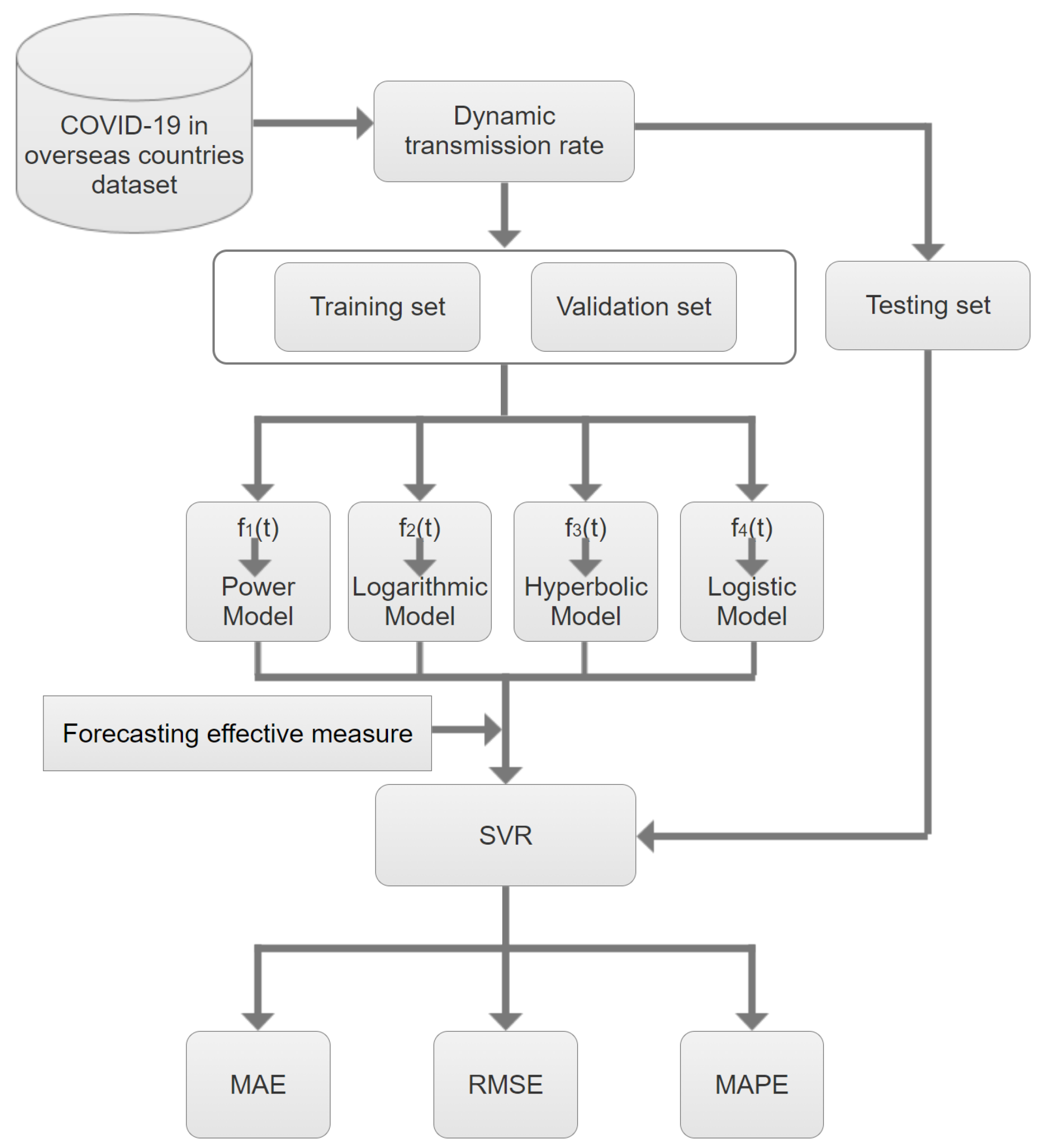
The forecasting framework of INCDTRM is carried out in seven main stages, that are shown in Figure 1 and explained below.

Input Cumulative confirmed cases $L\left(t\right)$, Cumulative deaths $D\left(t\right)$, Cumulative cures $K\left(t\right)$, $t=1,2,\dots ,T$.

Output Estimates of the existing cases $\widehat{N}\left(t\right)$, $t=T+1,T+2,\dots$.

Step 1. Calculating the existing cases $N\left(t\right)=L\left(t\right)-K\left(t\right)-D\left(t\right)$, $t=1,2,\dots ,T$.

Step 2. Choosing the best sliding window period k.

Step 3. Calculating $h_t$ using Equations (3) and (4), and divided the result into two parts. 3/4 sub-sets are used as the training set where time $t=k,k+1,\dots ,m$ and the remaining sub-sets are devoted as the validation set, $t=m+1,\dots ,T$.

Step 4. Fitting the training set based on four fitting functions $f_i\left(t\right)$ ($i=1,2,3,4$), and getting the estimated dynamic transmission rate ${\widehat{h}}_{it}$,$t=[k,T]$

Step 5. Introducing ${\widehat{h}}_{it}$ ($t\in [k,m]$) into SVR, and using SVR to estimate the dynamic transmission rate ${\widehat{h}}_{it}$ ($t\in [k,T]$) corresponding to the validation set. Then selecting the optimal combined model based on FEM and SVR by Algorithm 1.

Step 6. Predicting the dynamic transmission rate from the optimal combined model $M_c$, and calculating the estimated number of existing cases using Equation (6) after the T-th periods, respectively.

Step 7. The performance of the model is determined by the mean absolute error (MAE), root mean square error (RMSE), and mean absolute percentage error (MAPE), which are given by

$$\begin{array}{c}\begin{array}{cc}\hfill MAE& ={\displaystyle \frac{1}{T}}\sum _{t=1}^T|N\left(t\right)-\widehat{N}\left(t\right)|,\hfill \end{array}\hfill \end{array}$$

(16)

$$\begin{array}{c}\begin{array}{cc}\hfill RMSE& =\sqrt{{\displaystyle \frac{1}{T}}\sum _{t=1}^T{(N\left(t\right)-\widehat{N}\left(t\right))}^2}\hfill \end{array}\hfill \end{array}$$

(17)

and

$$\begin{array}{c}\begin{array}{cc}\hfill MAPE& ={\displaystyle \frac{1}{T}}\sum _{t=1}^T\left|{\displaystyle \frac{N\left(t\right)-\widehat{N}\left(t\right)}{N\left(t\right)}}\right|\times 100\%,\hfill \end{array}\hfill \end{array}$$

(18)

respectively, where $\widehat{N}\left(t\right)$ and $N\left(t\right)$ are the estimated numbers of existing cases and actual numbers of existing cases, respectively.

It should be noted that in Step 6, training set and validation set are used to train the SVR and select the corresponding model parameters, respectively. Therefore, in the calculation of FEM, we consider the fitting ability and prediction ability of the model, which effectively avoids the overfitting of the model.

3. Results and Discussion

All our numerical experiments are carried out on a PC with AMD Ryzen 7 4800u CPU at 1.80 GHz and 16 GB of physical memory. The PC runs Python Version: 3.7.2 on Window 10 Enterprise 64-bit operating system, and the nonlinear fitting model and the SVR regression model are imported from the SVM class of sklearn python library and leastsq class of scipy python library.

3.1. Dataset Description

The COVID-19 data repository (https://github.com/CSSEGISandData/COVID-19, accessed on 17 September 2021) used in the study was obtained from the Johns Hopkins University Center for Systems Science and Engineering (JHU CSSE) [30]. In this paper, we consider the following countries: USA, Canada, Germany, Italy, France, Spain, South Korea and Iran. The cumulative confirmed cases and deaths in each country, as well as the period from the first and last reports, are listed in

Table 2. First and last report dates by country.

Continent	Country	Number of Observed Days	First Report	Last Report	Cumulative Confirmed Cases	Cumulative Deaths
North America	USA	111	28/01/2020	17/05/2020	1,507,773	90,113
North America	Canada	111	28/01/2020	17/05/2020	77,257	5801
Europe	Germany	111	28/01/2020	17/05/2020	176,369	7958
Europe	Italy	109	31/01/2020	17/05/2020	224,760	31,763
Europe	France	87	21/02/2020	17/05/2020	179,630	27,532
Europe	Spain	107	01/02/2020	17/05/2020	276,505	27,563
Asia	South Korea	111	31/01/2020	17/05/2020	11,050	262
Asia	Iran	89	19/02/2020	17/05/2020	120,198	6988

.

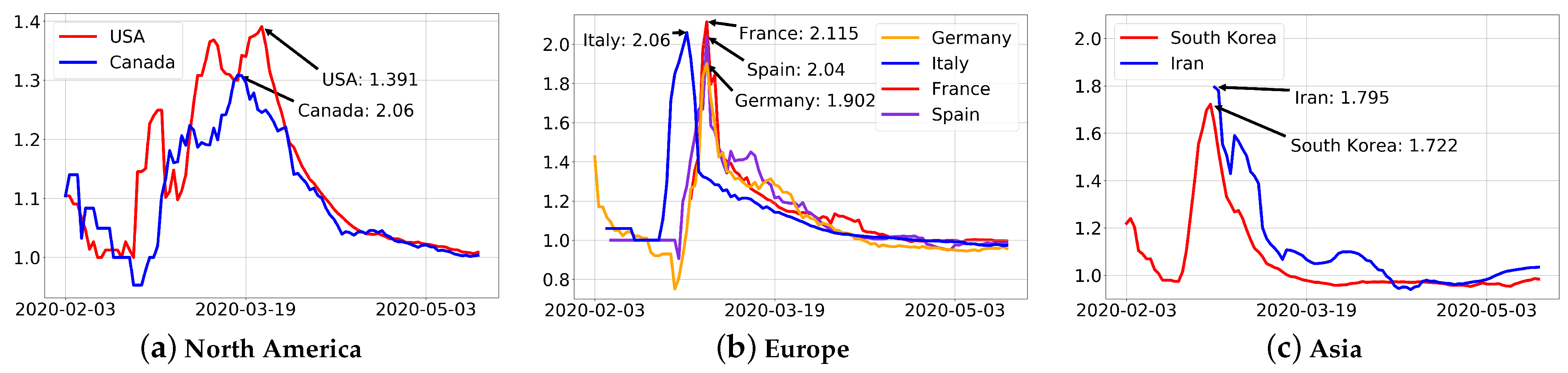
17 May 2020 is the end date of the first wave of the epidemic in most countries. When sliding window period is set to 7, the resulting dynamic transmission rates of the eight countries are shown in Figure 2.

Figure 2 shows that most countries experienced three stages, including a slow growth in the early stage, a rapid increase in the middle stage and a slow decline in the later stage. The experimental objects of this paper are mainly the third stage of overseas countries, i.e., the data after the dynamic transmission rate reaches the peak, and the subsets before 28 April 2020 are used to train the model to predict cases from 28 April 2020 to 17 May 2020. The data is normalized before training SVR and the normalized formula is given by

$$h_{it}^{*}=\frac{{\widehat{h}}_{it}-\min \left({\widehat{h}}_{it}\right)}{\max \left({\widehat{h}}_{it}\right)-\min \left({\widehat{h}}_{it}\right)}.$$

(19)

3.2. Choice of Sliding Window Period

The best sliding window period can effectively improve the prediction ability of the model. The basic idea of selecting the best sliding window period employed in this paper is to calculate the average mean absolute error (AVG_MAE) of four single models under different sliding window periods, and then determine the best sliding window period k according to the minimum AVG_MAE. The algorithm used for selecting the sliding window period in this paper is given in Algorithm 2 below.

Algorithm 2 Selecting the best sliding window period

Input: Existing cases $N\left(t\right)$, $t=1,2,\dots ,T$ Output: The best sliding window period k 1: begin 2: Divide the data into two parts, a training set where $t=1,2,\dots ,N-7$ and a testing set where $t=T-6,T-5,\dots ,T$. 3: for$k=1\to 7$do 4:     Evaluate the dynamic transmission rate using Equations (3) and (4) with the training set. 5:     Built four prediction models using Equation (5). 6:     Predict the dynamic transmission rate using four single models $f_i\left(t\right),i=1,2,\dots ,4$, and evaluate the estimated values of existing cases using (6), $t=T-6,T-5,\dots ,T$. 7:     Evaluate the MAE of the four models using Equation (16), and calculate AVG_MAE. 8: end for 9: return min(AVG_MAE) → best k

Using Algorithm 2, we obtain the best sliding window periods for eight countries (

Table 3. The best sliding window period.

Country	Best k
USA	7
Canada	4
Germany	2
Italy	7
France	4
Spain	2
South Korea	1
Iran	1

). The results show that the best sliding window periods for North American and European countries are larger than those for Asia. The result is attributed to the sliding window period being capable of effectively suppressing data fluctuations due to the large numbers of existing cases in North American and European countries.

3.3. Weight and Parameters Setting in SVR

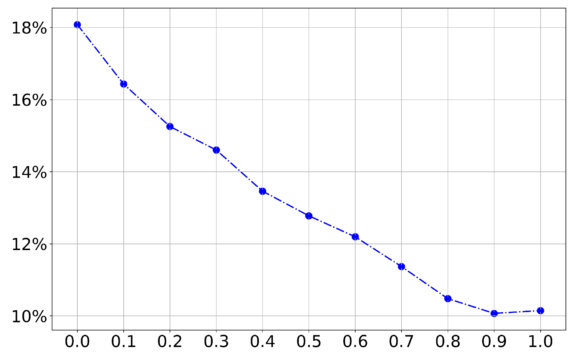
Reasonable parameters for SVR can effectively improve the model’s fitting and predictive ability. In this paper, we use the grid search to select the weight $\lambda$ of the combined kernel function, and Figure 3 shows the average MAPE of the epidemic prediction in eight countries under different weights $\lambda$.

It can be seen from Figure 3 that with the increase of weight, the average MAPE shows a decreasing trend, and when the weight is 0.9, the predicted average MAPE takes the minimum value, so the weight of the combined kernel function is set to 0.9 in this paper.

In addition, the particle swarm optimization (PSO) algorithm is used to search the optimal parameters for SVR. The initial values of the parameters in the PSO algorithm are set as shown in

Table 4. Parameters search range.

Parameters	Min	Max
C	0.1	1
$\gamma$	0.1	1

and the results are displayed in

Table 5. Parameter values.

Country	C	$\mathit{\gamma }$	$\mathit{\epsilon }$
USA	0.2370	0.9997	0.0001
Canada	0.1000	0.3817	0.0001
Germany	0.3000	0.9387	0.0001
Italy	0.2050	0.5301	0.0001
France	1.0000	0.1728	0.0001
Spain	0.1555	1.0000	0.0001
South Korea	0.6988	0.5003	0.0001
Iran	1.0000	0.1950	0.0001

.

3.4. Comparative Analysis of Different Models

To verify the validity of each model, we present the experimental results in detail in this subsection; at the same time, we also compare the performance results of our proposed method with the six different regression models, including four single methods, DGRM [19], and nonlinear combinational dynamic transmission rate model (NCDTRM). In

Table 6. Forecast accuracy of different models.

Country	Criteria	Model
		${\mathit{f}}_{\mathbf{1}}\left(\mathit{t}\right)$	${\mathit{f}}_{\mathbf{2}}\left(\mathit{t}\right)$	${\mathit{f}}_{\mathbf{3}}\left(\mathit{t}\right)$	${\mathit{f}}_{\mathbf{4}}\left(\mathit{t}\right)$	DGRM [19]	NCDTRM [20]	INCDTRM
	MAE	181,553.51	203,871.45	86,416.17	39,651.20	181,553.51	32,902.72	12,068.99
USA	RMSE	213,320.96	239,621.02	100,376.01	57,410.14	21,3320.96	48,042.41	16,261.69
	MAPE	17.91%	20.11%	8.54%	3.83%	17.91%	3.18%	1.20%
	MAE	2794.54	7550.63	5460.93	2077.57	2452.26	1160.59	1007.98
Canada	RMSE	3345.02	8740.13	6285.81	2267.68	2973.74	1320.66	1300.06
	MAPE	8.63%	23.37%	16.91%	7.39%	7.56%	3.59%	3.11%
	MAE	4067.54	2377.99	1784.45	1784.76	4996.27	2717.74	1595.88
Germany	RMSE	4871.16	3044.10	2028.51	2028.81	5505.85	3374.36	1782.99
	MAPE	22.33%	13.21%	7.70%	7.70%	26.24%	15.10%	7.81%
	MAE	13,804.08	18,131.27	6579.78	6580.14	13,804.08	3763.30	3509.84
Italy	RMSE	14,792.03	19,482.71	8047.19	8047.59	14,792.03	4104.03	3856.71
	MAPE	16.13%	21.24%	8.03%	8.03%	16.13%	4.27%	3.97%
	MAE	32,738.55	36,091.83	15,380.00	15,378.93	28,154.59	9239.81	15,694.11
France	RMSE	37,108.48	40,924.42	18,531.11	18,529.96	32,288.02	11,827.25	19,165.06
	MAPE	35.16%	38.77%	16.53%	16.53%	30.25%	9.93%	16.87%
	MAE	16,646.87	22,236.10	16,259.88	16,259.61	8,681.20	10,815.32	5910.42
Spain	RMSE	20,180.09	26,274.62	19,429.43	19,429.11	9,974.91	11,061.34	6619.12
	MAPE	26.48%	35.21%	25.80%	25.80%	12.95%	15.85%	8.66%
	MAE	237.76	207.44	104.72	54.87	194.70	48.07	46.15
South Korea	RMSE	277.01	247.12	133.12	74.67	225.65	61.45	57.95
	MAPE	22.82%	20.05%	10.20%	5.34%	18.59%	4.62%	4.42%
	MAE	7622.71	6945.72	5692.07	4353.94	7667.84	5104.99	5534.86
Iran	RMSE	9134.48	8412.68	7103.17	5715.05	9040.22	6613.54	7046.04
	MAPE	48.41%	43.96%	35.72%	26.95%	48.85%	31.72%	34.55%
	AVG_MAPE	24.73%	26.99%	16.18%	12.70%	22.31%	11.03%	10.07%

, we present the predictive performance on the testing set of seven models (from 28 April 2020 to 17 May 2020). Table 6 shows that INCDTRM achieves the best results in multiple countries, followed by NCDTRM, and both combinational models obtain better prediction performance than single models. The MAPEs of INCDTRM are calculated as 1.20%, 3.11%, 7.81%, 3.97%, 8.66%, and 4.42% for USA, Canada, Germany, Italy, Spain and South Korea, respectively. These results illustrate the accuracy of INCDTRM in estimating the number of existing COVID-19 daily cases. Among them, the MAE and RMSE of INCDTRM are the smallest for Germany, but the MAPE is larger than that of the model $f_4\left(t\right)$. This is because when INCDTRM is used to predict the epidemic in Germany, the date with the largest number of existing cases is relatively accurate, but the date of the smallest number of existing cases has a larger prediction error.

Although the prediction accuracy of INCDTRM is not as good as that of SVR when predicting the epidemic pattern in USA and Iran, the overall accuracy of INCDTRM is better than that of the other six models, and the AVG_MAPE of INCDTRM is 10.07%, indicating the reliability and feasibility of the FEM in selecting the optimal sub-model.

It should be noted that when forecasting the epidemic pattern in France and Iran, all models perform very poorly. This situation occurs because the number of confirmed cases in these two countries has unpredictably increased and second wave of the epidemic has appeared. Moreover, the fitting functions used in this paper are all monotonically decreasing functions. If the predicted country has a second wave of the epidemic, i.e., the dynamic transmission rate increases instead of decreasing, then all models in this paper will fail. This is the defect of this type of model.

3.5. Inflection Point Prediction

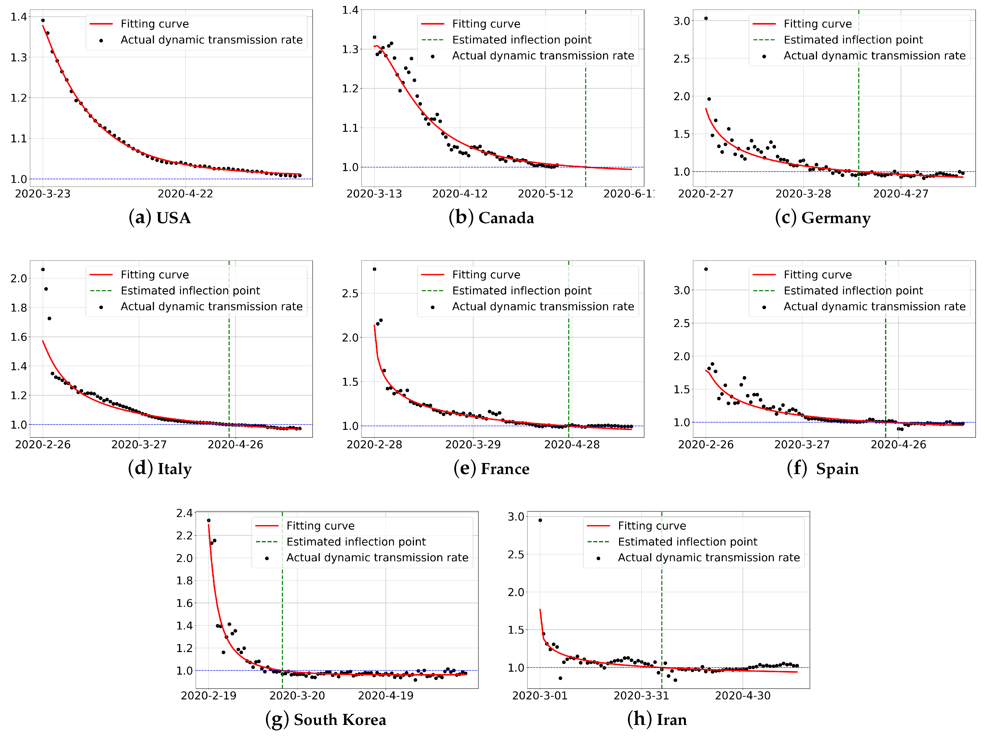
In this subsection, we estimate the inflection points of the epidemics in these countries. The definition of the inflection point is that the number of existing cases does not increase until it starts to decline, i.e., the dynamic transmission rate is equal to 1 [18]. The epidemic has the following properties around the inflection point: Before the inflection point, the epidemic is at an increasing stage; at the inflection point, the epidemic has the greatest pressure on the prevention and the medical system; after the inflection point, the epidemic situation has eased, and the pressure on prevention and control has gradually reduced. The emergence of an inflection point indicates that the number of existing infections has reached the maximum and has since been declining, which means that the epidemic is turning from bad to good. Using this model to estimate the inflection point of the epidemic can provide a reference value for understanding the epidemic spreading trend and can guide the timely release of relevant policies. The results are displayed in

Table 7. The inflection point.

Country	Estimated Inflection Point	Actual Inflection Point
USA	04/08/2020	31/05/2020
Canada	26/05/2020	31/05/2020
Germany	14/04/2020	08/04/2020
Italy	24/04/2020	20/04/2020
France	27/04/2020	16/04/2020
Spain	22/04/2020	25/04/2020
South Korea	15/03/2020	12/03/2020
Iran	06/04/2020	05/04/2020

and Figure 4.

Figure 4 shows that there is a delay between the estimated inflection point and the actual inflection point. This due to the fact that the model introduces the sliding window period k, which delays the transmission and updating of information, and the delay increases with the size of the sliding window period. However, most of the inflection point estimation errors are within one week.

Figure 4a,b show that the epidemic spread in North American countries is relatively late. The fitting curve of USA is relatively flat, but the change in the dynamic transmission rate from 22 April 2020 to 27 April 2020 is very small, and the decline in the curve is not obvious in the subsequent prediction, which is approximately a straight line, and resulting in a backward estimate of the inflection point. The outbreak in Canada fluctuate considerably, but overall shows a downward trend, and the inflection point is estimated in 26 May 2020.

Figure 4c–f show that European countries do not pay enough attention to the epidemic in the early stages, and the epidemic spread more rapidly, meaning that the dynamic transmission rate is larger. Then, with the subsequent strengthening of the prevention and control measures, the epidemic trend improves. Finally, the inflection points of Germany, Italy, France and Spain are estimated in 14 April 2020, 24 April 2020, 27 April 2020 and 22 April 2020, respectively. It should be noted that the dynamic transmission rate of France hovered in Annex 1 from 15 April to 27 April, which led to the delay of the estimated inflection point.

Figure 4g,h show that in the epidemic curves for South Korea and Iran, the declines are larger in the early days, meaning that the slopes of the curves are comparatively large. This is mainly due to the two countries implementing strong prevention and control measures in the early stages, and the epidemic situation is quickly brought under control. The inflection points for South Korea and Iran are estimated to be 14 March 2020 and 5 April 2020, respectively, earlier than those for European and North American countries. However, the outbreak in Iran rebounds again in May, and this is the main reason for the relatively large error in the forecast.

3.6. Sensitivity Analysis

Due to the deviation of epidemic statistics and the lag of data updating in various countries, whether the prediction model can effectively resist noise, that is, the impact of small changes in the original data on the output of the model, is also an important evaluation index in this paper.

The data is processed as follows: the daily number of existing cases is randomly added or reduced by 0–1% of its own value. Then the output of the model is compared with the output of the original model, and the formula of relative change rate is as follows:

$$\begin{array}{c}\begin{array}{c}\hfill \tilde{Q}={\displaystyle \frac{1}{T}}\sum _{t=1}^T\left|{\displaystyle \frac{\tilde{N}\left(t\right)-\widehat{N}\left(t\right)}{\widehat{N}\left(t\right)}}\right|\times 100\%,\end{array}\hfill \end{array}$$

(20)

where $\tilde{N}\left(t\right)$ and $\widehat{N}\left(t\right)$ represent the output of the noise model and the output of the original model, respectively. Each country has done 10 experiments, and the experimental results are shown in the form of average ± standard deviation.

As shown in

Table 8. First and last report dates by country.

Country	Dynamic Transmission Rate	The Existing Number of Cases
USA	0.16% ± 0.09%	1.65% ± 1.05%
Canada	0.14% ± 0.06%	1.31% ± 0.50%
Germany	0.30% ± 0.22%	3.46% ± 2.74%
Italy	0.24% ± 0.28%	2.76% ± 3.19%
France	0.25% ± 0.09%	3.03% ± 1.18%
Spain	0.23% ± 0.15%	2.18% ± 1.44%
South Korea	0.25% ± 0.16%	2.56% ± 1.64%
Iran	0.22% ± 0.17%	2.14% ± 1.69%

, in terms of dynamic transmission rate, the average rate of change in all countries is less than 0.3%. Except Germany and France, all average variabilities of the existing number of cases in other countries are not greater than 3%. For Germany, the fluctuation of the early dynamic transmission rate is obvious, and the later dynamic transmission rate fluctuates periodically (as shown in Figure 4), which are the reasons for the larger average rate of change. It is noteworthy that the standard deviation of the change rate in the existing number of cases in Italy is greater than that in Germany, but the average ± standard deviation is better than that in Germany. The average change rate of the dynamic transmission rate in all experiments was smaller than that of the existing infected population. This is because that the base number of the existing cases was large, and the small change of the dynamic transmission rate would cause large changes in the existing infected population. On the whole, our model has good anti-noise ability and stability when dealing with data fluctuations.

3.7. Global Epidemic Forecast

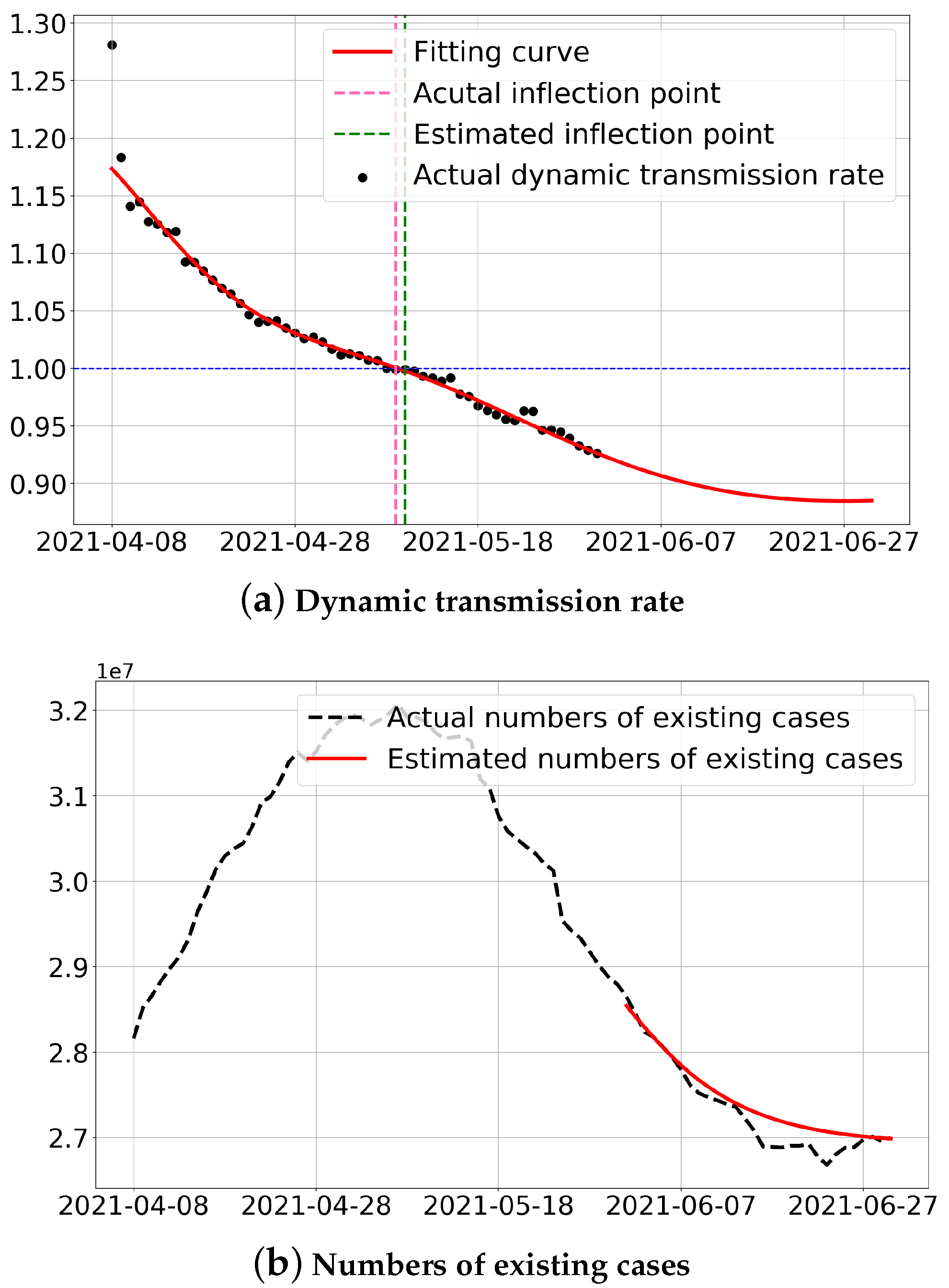
Accurate prediction of the global epidemic is the key to effectively grasping the overall trend of the COVID-19 pandemic. Based on the high performance of INCDTRM, we analyze and forecast the global epidemic. Since the global epidemic database is large and the data period is long, the late dynamic transmission rate is almost linear, and we do not have the ability to predict it. Therefore, the data are preprocessed as follows. First, we select the data from 1 April to 30 June 2021. Then, the existing case sequence is calculated, and the sequence is subtracted from the number of the existing cases on 31 March 2021. Finally, we take the sequence as experimental dataset. Figure 5 shows the development trend of the global epidemic in the future using INCDTRM.

As shown in Figure 5a, the spread of the global epidemics is falling, but with the increase of time, the declining trend of the global dynamic transmission rate begins to slow down. The inflection point is predicted as 10 May 2021, in which the actual inflection point was 9 May 2021, indicating that the model in this paper has high reliability. In addition, the number of existing infections is predicted in the global epidemic from 1 June to 30 June 2021, a total of 30 days. In Figure 5b, the number of existing infections in the global epidemic is decreasing, and the estimated number of existing cases is consistent with the actual trend of the number of existing cases. The estimated errors of MAE, RMSE and MAPE are 141,374.15, 182,765.24 and 0.522%, respectively.

However, the number of existing infections in the global epidemic fluctuated in June 2021. Therefore, we should continue to appeal to wear masks and stop large-scale gatherings to avoid the rebound of the epidemic trend. At the same time, the development of a vaccine for COVID-19 is also an effective way to effectively suppress the spread of infectious diseases [31]. In addition, we can update the prediction model in real time according to the daily new data, and thus we can grasp the spread trend of global epidemics in a timely manner.

4. Conclusions

In this paper, we have presented an INCDTRM based on FEM and SVR for analyzing and predicting the COVID-19 pandemic in eight countries. The experimental results show that INCDTRM has smaller prediction error and stronger generalization ability than the single prediction models, DGRM and NCDTRM that have been used previously; forecast errors for epidemics in USA, Canada, Italy and South Korea were within 5%. This shows the rationality of using dynamic transmission rate to replace the basic infection number $R_0$, and our model can thus be utilized for predicting the COVID-19 epidemic.

Furthermore, we also used INCDTRM to model the global COVID-19 pandemic. The experimental results predict that the inflection point of the global epidemic is May 10, 2021. and the estimated errors of MAE, RMSE and MAPE are 141,374.15, 182,765.24 and 0.522%, respectively. As Ferguson et al. [32] pointed out that we are now at a critical moment of the epidemic, and any slackening in prevention and control will lead to a rebound in the spread of the epidemic.

It should be noted that this paper has the following defects: (1) Due to the monotonicity of the fitting functions, INCDTRM is not suitable for predicting a rebound in an epidemic; (2) The weights of the combined kernel function and the initial parameters of PSO need to be set according to experience; (3)The spread of COVID-19 epidemic is affected by social factors [33], population [34], climate, environment [35] and other factors, which is very complex, but this paper only considers a single epidemic data, without considering other factors that may affect the spread of the epidemic.

According to the above limitations, the future work of this paper is as follows: (1) Finding a suitable COVID-19 multi-stage infectious disease development model; (2) Using more effective multi kernels learning models and adaptive optimization algorithms; (3) We will further collect relevant data and conduct research with data assimilation or SEIR and its extended model.

References

- WHO Director-General, World Health Organization. 11 February 2020. Available online: https://www.who.int/director-general/speeches/detail/who-director-general-s-remarks-at-the-media-briefing-on-2019-ncov-on-11-february-2020 (accessed on 17 September 2021).
- Yang, Z.; Zeng, Z.; Wang, K.; Wong, S.S.; Liang, W.; Zanin, M.; Liu, P.; Cao, X.; Gao, Z.; Mai, Z.; et al. Modified SEIR and ai prediction of the epidemics trend of COVID-19 in China under public health interventions. J. Thorac. Dis. 2020, 12, 165–174. [Google Scholar] [CrossRef] [PubMed]
- Wu, J.; Leung, K.; Leung, G. Nowcasting and forecasting the potential domestic and international spread of the 2019-nCoV outbreak originating in Wuhan, China: A modelling study. Lancet 2020, 395, 689–697. [Google Scholar] [CrossRef] [Green Version]
- Lopez, L.; Rodo, X. A modified SEIR model to predict the COVID-19 outbreak in Spain and Italy: Simulating control scenarios and multi-scale epidemics. Results Phys. 2021, 21, 103746. [Google Scholar] [CrossRef] [PubMed]
- Mahajan, A.; Sivadas, N.; Solanki, R. An epidemic model SIPHERD and its application for prediction of the spread of COVID-19 infection in India. Chaos Solitons Fractals 2020, 140, 110156. [Google Scholar] [CrossRef]
- Sanyi, T.; Biao, T.; Bragazzi, N.L.; Fan, X.; Tangjuan, L.; Sha, H.; Pengyu, R.; Xia, W.; Xiang, C.; Zhihang, P.; et al. Analysis of COVID-19 epidemic traced data and stochastic discrete transmission dynamic model. Sci. Sin. Math. 2020, 50, 1071. (In Chinese) [Google Scholar]
- Ankarali, H.; Ankarali, S.; Caskurlu, H.; Cag, Y.; Arslan, F.; Erdem, H.; Vahaboglu, H. A statistical modeling of the course of COVID-19 (SARS-CoV-2) outbreak: A comparative analysis. Asia-Pac. J. Public Health 2020, 32. [Google Scholar] [CrossRef]
- Liu, Z. Uncertain growth model for the cumulative number of COVID-19 infections in China. Fuzzy Optim. Decis. Mak. 2020, 20, 229–242. [Google Scholar] [CrossRef]
- Smirnova, A.; DeCamp, L.; Chowell, G. Mathematical and Statistical Analysis of Doubling Times to Investigate the Early Spread of Epidemics: Application to the COVID-19 Pandemic. Mathematics 2021, 9, 625. [Google Scholar] [CrossRef]
- Parbat, D.; Chakraborty, M. A python based support vector regression model for prediction of COVID19 cases in India. Chaos Solitons Fractals 2020, 138, 109942. [Google Scholar] [CrossRef]
- Tuli, S.; Tuli, S.; Tuli, R.; Buyya, R. Predicting the growth and trend of COVID-19 pandemic using machine learning and cloud computing. Internet Things 2020, 11, 100222. [Google Scholar] [CrossRef]
- Zeroual, A.; Harrou, F.; Dairi, A.; Sun, Y. Deep learning methods for forecasting COVID-19 time-series data: A comparative study. Chaos Solitons Fractals 2020, 140, 110121. [Google Scholar] [CrossRef] [PubMed]
- Devaraj, J.; Elavarasan, R.M.; Pugazhendhi, R.; Shafiullah, G.M.; Ganesan, S.; Jeysree, A.K.; Khan, I.A.; Hossain, E. Forecasting of COVID-19 cases using deep learning models: Is it reliable and practically significant? Results Phys. 2021, 21, 103817. [Google Scholar] [CrossRef]
- Bezerra, A.; Santos, E. Prediction the daily number of confirmed cases of COVID-19 in Sudan with ARIMA and holt winter exponential smoothing. Int. J. Dev. Res. 2020, 10, 39408–39413. [Google Scholar]
- González, P.; Núñez, C.; Sánchez, J.; Valverde, G.; Velasco, J. Expert System to Model and Forecast Time Series of Epidemiological Counts with Applications to COVID-19. Mathematics 2021, 9, 1485. [Google Scholar] [CrossRef]
- Layne, S.; Hyman, J.; Morens, D.; Taubenberger, J. New coronavirus outbreak: Framing questions for pandemic prevention. Sci. Transl. Med. 2020, 12, eabb1469. [Google Scholar] [CrossRef] [Green Version]
- Huang, E.; Qiao, F. A data driven time-dependent transmission rate for tracking an epidemic: A case study of 2019-nCoV. Sci. Bull. 2020, 65, 425–427. [Google Scholar] [CrossRef]
- Hu, Y.; Liu, Y.; Wu, L.; Wang, J.; Kong, J.; Zhang, Y.; Dai, Y.; Yang, Z. A dynamic transmission rate model and its application in epidemic analysis. Oper. Res. Trans. 2020, 24, 27–42. (In Chinese) [Google Scholar]
- Hu, Y.; Liu, Y.; Wu, L.; Wang, J.; Kong, J.; Zhang, Y.; Dai, Y.; Yang, Z. A dynamic growth rate model and its application in global COVID-19 epidemic analysis. Acta Math. Appl. Sin. 2020, 43, 452–467. (In Chinese) [Google Scholar]
- Xie, X.; Luo, K.; Zhang, Y.; Jin, J.; Lin, H.; Wang, G. Nonlinear combinational dynamic transmission rate model and COVID-19 epidemic analysis and prediction in China. Oper. Res. Trans. 2021, 25, 17–30. (In Chinese) [Google Scholar]
- Chen, Y.; Xu, P.; Chu, Y.; Li, W.; Wu, Y.; Ni, L.; Bao, Y.; Wang, K. Short-term electrical load forecasting using the support vector regression (SVR) model to calculate the demand response baseline for office buildings. Appl. Energy 2017, 195, 659–670. [Google Scholar] [CrossRef]
- Wei, C. Chaotic particle swarm optimization algorithm in a support vector regression electric load forecasting model. Energy Convers. Manag. 2009, 50, 105–117. [Google Scholar]
- Yang, W.; Deng, M.; Xu, F.; Wang, H. Prediction of hourly PM2.5 using a space-time support vector regression model. Atmos. Environ. 2018, 181, 12–19. [Google Scholar] [CrossRef]
- Moser, G.; Serpico, S. Automatic parameter optimization for support vector regression for land and sea surface temperature estimation from remote sensing data. IEEE Trans. Geosci. Remote. Sens. 2009, 47, 909–921. [Google Scholar] [CrossRef]
- Smola, A.; Scholkopf, B. A tutorial on support vector regression. Stat. Comput. 2004, 14, 199–222. [Google Scholar] [CrossRef] [Green Version]
- Vapnik, V.N. Statistical Learning Theory; John Wiley & Sons: New York, NY, USA, 1998. [Google Scholar]
- Peng, Y.; Nagata, M. An empirical overview of nonlinearity and overfitting in machine learning using COVID-19 data. Chaos, Solitons Fractals 2020, 139, 110055. [Google Scholar] [CrossRef] [PubMed]
- Ribeiro, M.; Coelho, L. Ensemble approach based on bagging, boosting and stacking for short-term prediction in agribusiness time series. Appl. Soft Comput. 2020, 86, 105837. [Google Scholar] [CrossRef]
- Chen, Y.; Hou, D. Combination forecasting model based on forecasting effective measure with standard deviate. J. Syst. Eng. 2003, 18, 203–210, 223. (In Chinese) [Google Scholar]
- Dong, E.; Du, H.; Gardner, L. An interactive web-based dashboard to track COVID-19 in real time. Lancet Infect. Dis. 2020, 20, 533–534. [Google Scholar] [CrossRef]
- Lv, W.; Ke, Q.; Li, K. Dynamical analysis and control strategies of an SIVS epidemic model with imperfect vaccination on scale-free networks. Nonlinear Dyn. 2020, 99, 1507–1523. [Google Scholar] [CrossRef] [Green Version]
- Wang, H.; Wang, Y.; Walker, P.G.; Walters, C.; Winskill, P.; Whittaker, C.; Donnelly, C.A.; Riley, S.; Ghani, A.C. Impact of non-pharmaceutical interventions (NPIs) to reduce COVID-19 mortality and healthcare demand. Br. Med J. 2020. [Google Scholar]
- Lin, R.; Lin, S.; Yan, N.; Huang, J. Do prevention and control measures work? Evidence from the outbreak of COVID-19 in China. Cities 2021, 118, 103347. [Google Scholar] [CrossRef] [PubMed]
- Bhadra, A.; Mukherjee, A.; Sarkar, K. Impact of population density on Covid-19 infected and mortality rate in India. Model. Earth Syst. Environ. 2021, 7, 623–629. [Google Scholar] [CrossRef]
- Xu, X.; Zhang, X.; Mendes, J. Impacts of preference and geography on epidemic spreading. Phys. Rev. E 2007, 76, 056109. [Google Scholar] [CrossRef] [PubMed] [Green Version]
Figure 1.
Forecasting framework of INCDTRM.