COVID-19 Outbreak and CO2 Emissions: Macro-Financial Linkages


1
IPAG Lab, IPAG Business School, 184 boulevard Saint-Germain, 75006 Paris, France
2
Economics Department, Université Paris 8 (LED), 2 rue de la Liberté, 93526 Saint-Denis CEDEX, France
J. Risk Financial Manag. 2021, 14(1), 12; https://doi.org/10.3390/jrfm14010012
Submission received: 4 December 2020
/
Revised: 22 December 2020
/
Accepted: 24 December 2020
/
Published: 29 December 2020
(This article belongs to the Special Issue Energy Finance and Sustainable Development)
Abstract
:In the Dynamic Conditional Correlation with Mixed Data Sampling (DCC-MIDAS) framework, we scrutinize the correlations between the macro-financial environment and CO emissions in the aftermath of the COVID-19 diffusion. The main original idea is that the economy’s lock-down will alleviate part of the greenhouse gases’ burden that human activity induces on the environment. We capture the time-varying correlations between U.S. COVID-19 confirmed cases, deaths, and recovered cases that were recorded by the Johns Hopkins Coronavirus Center, on the one hand; U.S. Total Industrial Production Index and Total Fossil Fuels CO emissions from the U.S. Energy Information Administration on the other hand. High-frequency data for U.S. stock markets are included with five-minute realized volatility from the Oxford-Man Institute of Quantitative Finance. The DCC-MIDAS approach indicates that COVID-19 confirmed cases and deaths negatively influence the macro-financial variables and CO emissions. We quantify the time-varying correlations of CO emissions with either COVID-19 confirmed cases or COVID-19 deaths to sharply decrease by −15% to −30%. The main takeaway is that we track correlations and reveal a recessionary outlook against the background of the pandemic.
Keywords:
COVID-19; CO2 emissions; time-varying correlations; macroeconomy; stock markets; DCC MIDAS1. Introduction
With the quarantine in action in most industrialized countries since mid-March 2020, market observers predict a deep recession for 2021–2022. As Carlsson-Szlezak et al. (2020) put it, “COVID-19 risks have been priced so aggressively across various asset classes that some fear a recession in the global economy” (p. 2). Stock markets plunged in March–April 2020 as a direct consequence of the Coronavirus’s shocking news spreading around the world. Indeed, Baker et al. (2020) report that the U.S. stock market reacted so much more forcefully to COVID-19 than to previous pandemics, such as the Spanish Flu. Investor managers already document that the stock-bond correlation has been negatively affected by the COVID-19 outbreak (Papadamou et al. 2020).
A burgeoning literature is emerging on the COVID-19’s financial outcomes, whereby the role of fear and uncertainty plays a central role (Lyócsa and Molnár 2020). Baig et al. (2020) link COVID-19 cases/deaths, stock market volatility, and illiquidity. In the U.S., Albulescu (2020) demonstrates that the sanitary crisis enhanced the S&P 500 realized volatility. While using an Infectious Disease Equity Market Volatility Tracker (EMV-ID), Bai et al. (2020) further investigate the effects of infectious disease pandemic on the volatility of the U.S., China, U.K., and Japan stock markets. Rizwan et al. (2020) investigate how COVID-19 impacted the systemic risk in eight countries’ banking sectors (including China). Azimli (2020) focuses on the Google Search Index for Coronavirus (GSIC) and the risk-return dependence structure. Topcu and Gulal (2020) document the negative impact of the pandemic on emerging stock markets. Gharib et al. (2020) reveal the bilateral contagion effect of bubbles in oil and gold markets during the recent COVID-19 outbreak. Last but not least, Mazur et al. (2020) find that natural gas, food, healthcare, and software stocks earn high positive returns; whereas, equity values in petroleum, real estate, entertainment, and hospitality sectors fall dramatically. Similarly to the years 2007–2008, which provided an experience that most economists, practitioners, and policymakers never thought they would witness (Melvin and Taylor 2009), the year 2020 brought along the COVID-19 sanitary crisis. To some extent, this most recent phenomenon can be compared to the two previous financial crises, inherited, respectively, from the U.S. sub-primes defaults and the European debt hazards1
Kamin and DeMarco (2012) underline the failure of the banking industry in the wake of the Lehman Brothers’ collapse. Realizing that financial firms around the world were pursuing similar (flawed) business models2 was a hard hit on the banker’s consciousness and payroll. Similarly, governments and policymakers were underprepared to deal with a pandemic (such as respiratory equipment in hospitals or the mass production of disposable masks), as the World Health Organization rang the bell (Sohrabi et al. 2020).
Gruppe et al. (2017) review the literature on interest rate convergence and the European debt crisis with a particular focus on the fiscal problems of some countries (such as Greece) in Europe. Moro (2014) further details how the European economic and financial Great Crisis spread quickly among closely integrated economies, either through the trade channel or the financial channel. In that latter case, the solution would be found in a more effective political integration. This is precisely what the EU-27 is aiming at with the simultaneous distribution of the Pfizer-BioNTech COVID-19 and Moderna vaccines across the member countries as early as 27 December 2020 as well as in the early days of 2021 (National Academies of Sciences 2020).
In the meantime, the issue of decreasing CO emissions is attached to the lock-down, with the dramatic reduction in international trade and tourism that followed shipping routes’ and airports’ closure. The sanitary crisis and its associated uncertainty determine an economic contraction through direct (real) or indirect (financial) channels. Consequently, the CO emissions slowdown. In this paper, we aim at quantifying the correlations between epidemiological (daily) cases, macro- (monthly) financial (intra-daily) factors, and (monthly) CO emissions in the Dynamic Conditional Correlation with Mixed Data Sampling (DCC-MIDAS) framework (Colacito et al. 2011). Introduced by Ghysels et al. (2004), this technique allows mixing the data frequencies by resorting to lag polynomials and dedicated weight functions. Empirical studies relying on the DCC-MIDAS in the finance literature include to cite few, Asgharian et al. (2016) for the long-run stock-bond correlation, Conrad et al. (2014) for long-term correlations in U.S. stock and crude oil markets, or Xu et al. (2018) for measuring the systemic risk of the Chinese banking industry.
To our best knowledge, this piece of research is the first to study the correlations between COVID-19 epidemiological cases, macro-financial factors, and CO emissions. Our article’s interest is to visualize the correlations with the macro-financial environment due to COVID-19 clinical cases’ multiplication. U.S. cases of confirmed, dead, and recovered patients of COVID-19 are sourced from the Johns Hopkins Coronarirus Center3. U.S. macroeconomic indicators and CO emissions are sourced from the U.S. Energy Information Administration4. Tick-by-tick data for U.S. stock markets are accessed from the Oxford-Man Institute for Quantitative Finance5.
Extant literature on the link between CO emissions and the macroeconomy includes Chevallier (2011a, 2011b), who described the joint dynamics of industrial production and carbon prices by means of regime threshold vector error-correction and Markov-switching VAR models. Regarding correlations, more specifically, Chevallier (2012) documents time-varying correlations between energy markets (oil and gas) and CO. Lutz et al. (2013) examined the nonlinear relation between the E.U. carbon price and its fundamentals (such as energy prices, macroeconomic risk factors, and weather conditions) in a Markov regime-switching GARCH. Fell (2010) examines the dynamic relationship with Nordic wholesale electricity prices. Hintermann (2010) and Aatola et al. (2013) completed the analysis of CO price fundamentals based on structural modelling, Instrumental Variables, and Vector Auto-Regressive models.
Through the lens of correlations, we establish that COVID-19 confirmed cases and deaths have a negative and statistically significant influence on the macro-financial environment and CO emissions, i.e., there is a counter-cyclical business cycle pattern here. This result is precisely documented by the parameter governing the lag polynomials in MIDAS regressions and by the plots of long-run correlations. In the short run, we especially identify spikes in the stock market. Time-varying correlations between the COVID-19 and CO emissions are documented to drop dramatically by −15% to −30% depending on the underlying instrumental variable (i.e., COVID-19 confirmed cases or COVID-19 deaths). When introducing the number of COVID-19 recovered patients in the dynamic system of equations, we record, on the contrary, a positive sign for the MIDAS coefficient, which suggests that, with more patients healing, the U.S. economy is on track for a recovery. This latter result is only visible for one panel interacting COVID-19 recovered cases with industrial production, whereas correlations that stem from stock markets and CO emissions still paint a recessionary outlook.
2. Data
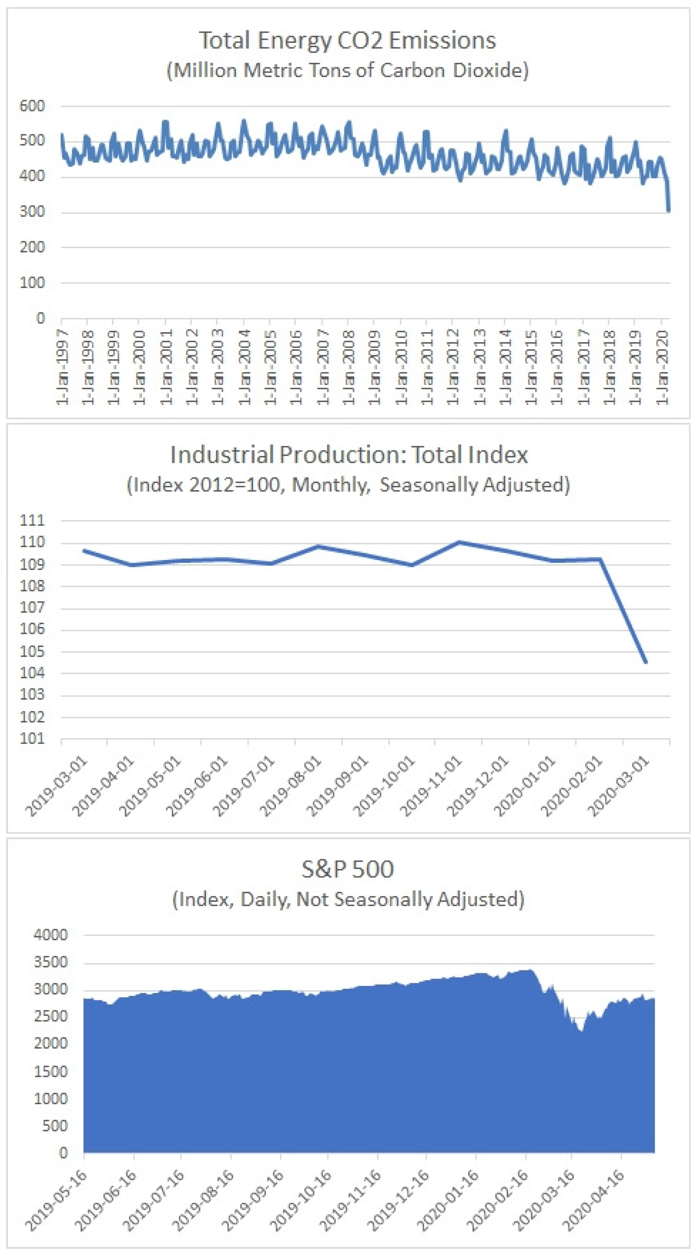
As a proteiform disease, COVID-19 is drowning the macro-financial environment into a recession that it is too early to foreshadow. Our study’s primary variable of interest is the U.S. growth rate of CO emissions, which is expected to decrease due to the pandemic. In order to fix ideas, we show our intuition in Figure 1, which extracts data from the U.S. Energy Information Administration and the Federal Reserve Bank of St. Louis. Year-on-year, it is visible that macroeconomic (as proxied by industrial production) and financial (as proxied by the S&P 500) factors took a severe blow since mid-March 2020.
2.1. U.S. COVID-19 Cases
For epidemiological cases, the U.S. time-series that were extracted from the Johns Hopkins Repository on 5 May 2020 are of (3×) kinds:
- confirmed cases,
- deaths, and
- recovered cases.
with a daily frequency. One-by-one, these variables will be considered in correlation models combining the CO emissions and macro-financial factors. At the time of writing, the USA totaled 1,309,550 confirmed cases; 78,795 deaths; and, 212,534 recovered cases. Because of data availability, we focus our article on the USA as a representative of the world. Indeed, for other countries, data on CO emissions dates back to the year 2017 at best. A snapshot of the U.S. time-series is given in Figure 2, revealing the worrying trend behind the pandemic.
Each panel displays Generalized Linear Models (GLM). The dispersion parameter for the “Poisson” family is set to 1. Fisher Scoring is the iteration measure used to fit the model.
2.2. U.S. Macroeconomic Indicators and CO Emissions
Another category of explanatory variables is contained in the U.S. Energy Information Administration database6 released in May 2020 (as part of the Short-Term Energy Outlook) monthly. This database contains the growth rate of CO emissions, as well as business cycle indicators that are linked to the state of the U.S. economy (see Table 1).
The indicators are listed according to the following sub-categories: macroeconomic indicators (11×), manufacturing production indices (14×), price indexes (4×), miscellaneous (5×), and, finally, CO emissions (4×).
This article chooses to work with the Total Industrial Production Index (that is representative of the macroeconomic factor) and the Total Fossil Fuels CO emissions variable. Additional specifications are discussed in the sensitivity analysis (Section 4.5).
2.3. U.S. Stock Markets
Finally, we encompass U.S. stock markets’ closing returns that are based on the Oxford ’Realized Library’ with an intra-daily frequency. Tick-by-tick data are sampled over the 5-min. horizon in order to avoid microstructure noise7. These variables are included to proxy for the financial markets’ downward trend and its correlation with CO emissions. Following the same logic as decreasing industrial production (e.g., freezing global economy) due to the COVID-19 pandemic, stock markets (such as the NYSE) briefly halted from trading in March 2020, and they have not recovered yet from the crash that ensued.
Table 2 details the list of assets.
In the main text, we run the estimates with S&P 500 as the financial factor. Other indexes can be included for robustness checks (Section 4.5).
2.4. Series’ Transformation
In order to ensure stationarity of the time-series, we use the growth rate of CO emissions indicator i at time t, diff the first-difference of the COVID-19 case type i, the growth rate of the macroeconomic indicator i, and the log-returns on the stock market i.8
3. Model
We consider the DCC-MIDAS by Colacito et al. (2011) in order to assess the time-varying correlations between COVID-19 epidemiological cases, macro-financial factors, and CO emissions. This class of Dynamic Conditional Correlation models obeys a DCC scheme by Engle and Sheppard (2001) for the daily dynamics, with, additionally, the correlations moving around a long-run component:
with the short-run correlation between assets i and j, the slowly moving long-run correlation, a normalization of cross-products for the standardized residuals , the computation of correlations, , and . is the vector of returns. is the vector of unconditional means. is the conditional covariance matrix. is the number of days that the long-run component (e.g., monthly macroeconomic variables) is held as fixed. The weighting scheme is similar to the GARCH-MIDAS (Engle et al. 2013):
with the number of lag polynomials of the MIDAS component, and the decay pattern across various series.
Equation (5) is known as the beta function weighting scheme. This procedure allows for estimating the number of lags for both the daily and monthly returns within MIDAS optimally. The setting of the MIDAS lags is detailed in the Appendix A for the interested reader. Ghysels et al. (2007) document that the beta function is a better choice than the exponential Almon when dealing with high-frequency data, as in our setting. It can produce various lag structures for past returns, such as monotonically increasing/decreasing or hump-shapes.
As is looked after by the researcher, the econometric system that is composed of Equations (1)–(5) can accommodate weights , lag lengths , and span lengths of historical correlations to differ across any pair of series.
The DCC-MIDAS is estimated by Two-Step Quasi Maximum Likelihood:
with the parameters of the conditional volatility being collected in a vector , and that of the conditional correlation into a vector . Splitting the log-likelihood function allows for firtst estimating the parameters of the conditional volatility while using , and second the DCC-MIDAS parameters with the standardized residuals using .
4. Results
4.1. Baseline Correlations (without COVID-19 Cases)
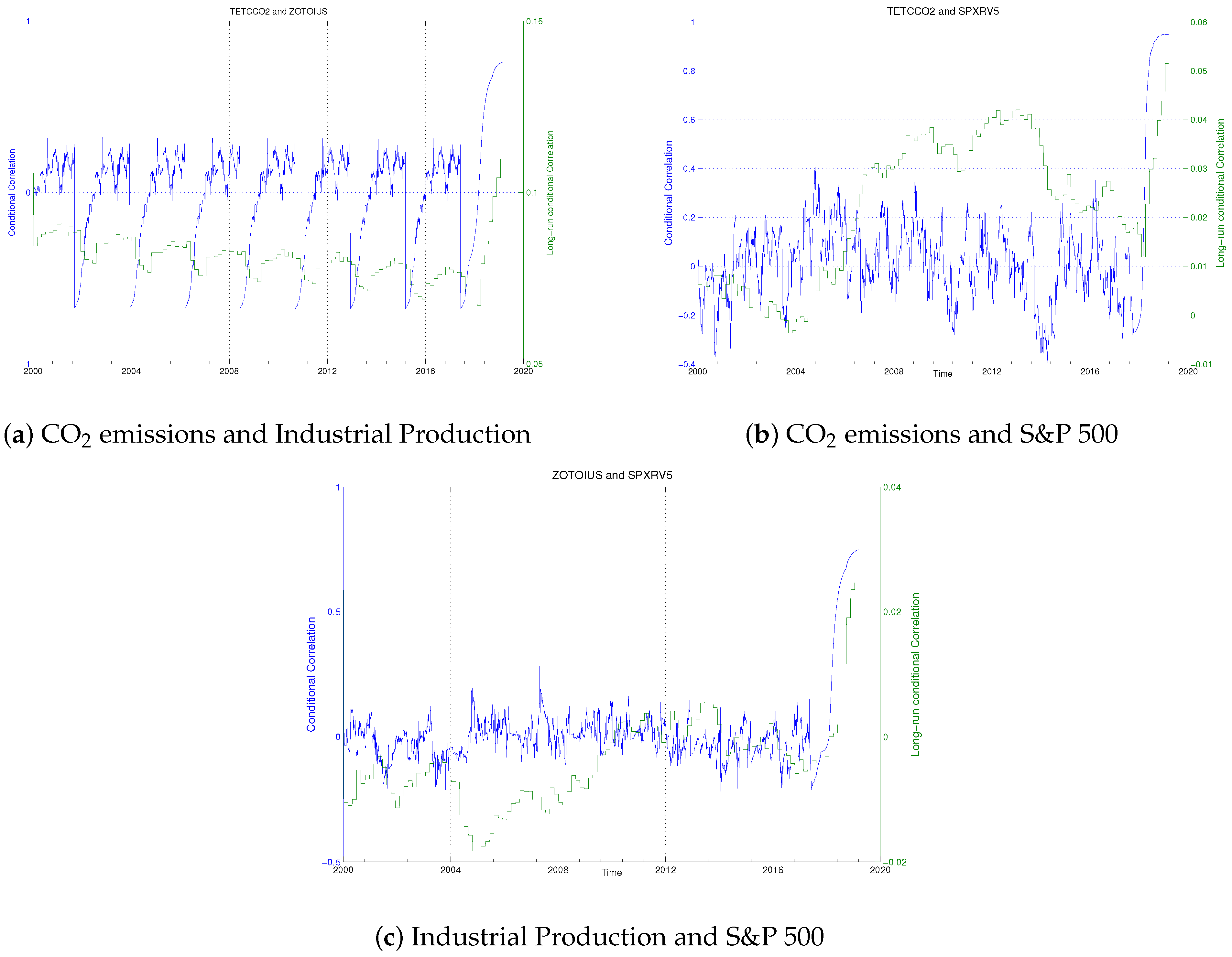
In this setting, we consider the Total Fossil Fuels CO emissions (), the Total Industrial Production Index (), and the 5-min. Realized Volatility of the S&P 500 Index () from 2000 to present.
GARCH-MIDAS and DCC-MIDAS parameter estimates are reproduced in Table 3, which reports the estimated parameters, standard errors, and the associated maximized log-likelihood values for the model under consideration.
In Table 3, for the GARCH-MIDAS part, and capture the short-term volatility dynamics, as in the ARCH and GARCH framework. We verify that they are statistically significant and positive. Plots of conditional variance have been saved to disk.9 The sum of is noticeably less than 1, i.e., the MIDAS-GARCH parameter is smaller than what is usually observed for conventional GARCH models.
Most of all, is strongly significant. In the baseline specification, a positive sign implies a positive relationship between the series at stake. In the context of the year 2020, we may interpret it as such: when industrial production decreases, the CO emissions decrease, and stock markets decline. Recall that, in a MIDAS regression, the lag polynomial coefficients are captured by a known function (e.g., the beta function in our case) of a few parameters that are summarized in a vector . The parameter determines the sign of the effect of the lagged on the long-term components.
The same logic applies to the DCC component’s comments, although the parameter here indicates the correlation level. Figure 3 shows the DCC-MIDAS conditional correlations (in blue) and long-run conditional correlations (in green) for the baseline specification. As a sign of financial contagion, the graphs pick up correlation increases near the end of the study period. This is all linked to a macro-financial recessionary outlook against the broader background of the COVID-19 pandemic, precisely the next empirical sections’ purpose.
4.2. Introducing COVID-19 Confirmed Cases
For the introduction of the COVID-19 confirmed cases into the baseline specification, we restrict the estimation window to the sample that was accessed from the Johns Hopkins Coronavirus Center, e.g., 22 January 2020 to 8 May 2020.
In Table 4, the same comments apply to the baseline specification regarding the GARCH-MIDAS. We focus our attention primarily on the parameter estimate of for , which is −28.49 with a standard error of 6.84 (therefore, highly significant).
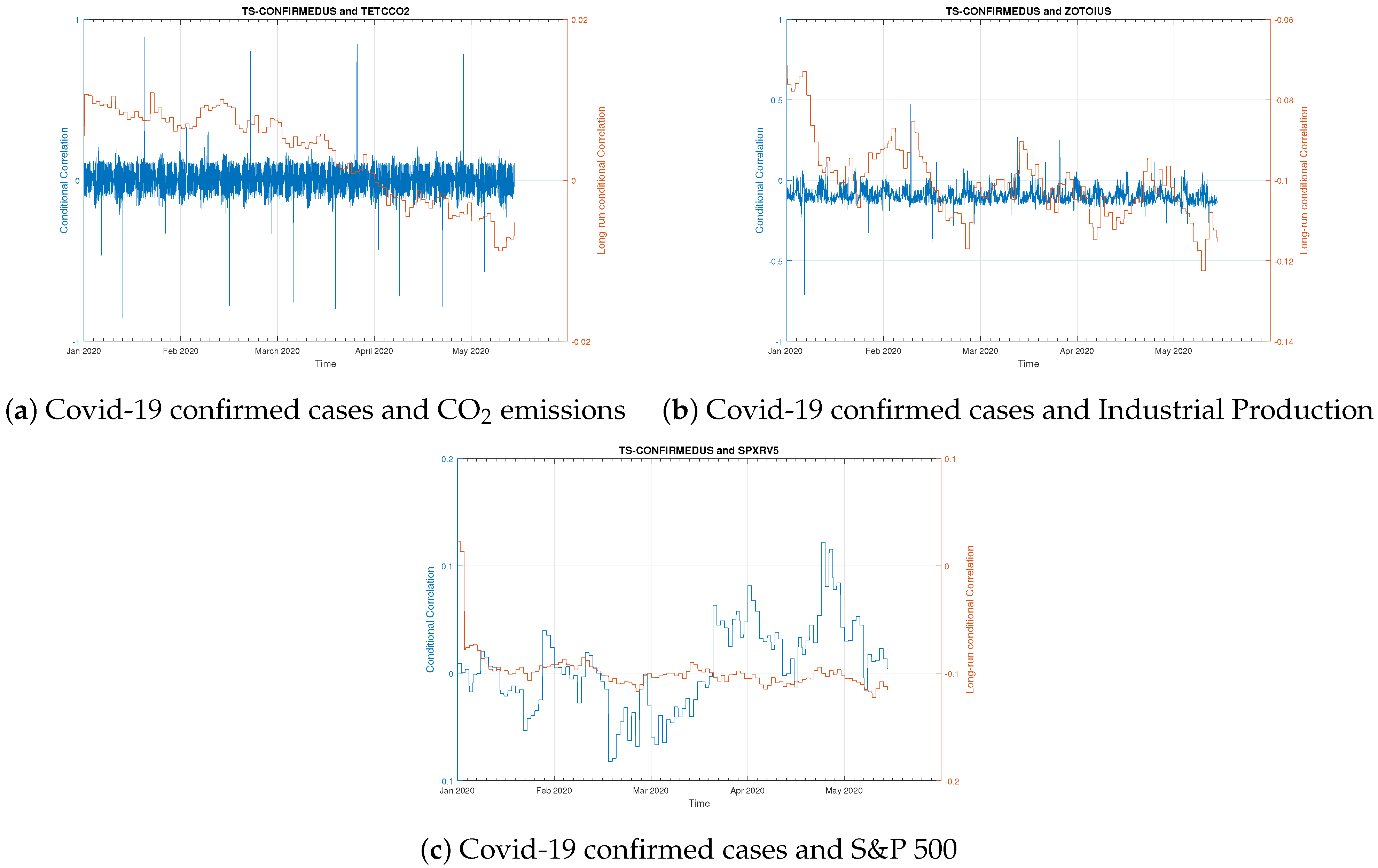
The negative sign for recorded here means that sharp increases of COVID-19 confirmed that cases in the U.S. had negatively influenced all other macro-financial and CO emissions variables. This is the first time, to our knowledge, that such a statement can be made from statistical expertise.
Figure 4 shows that all U.S. macro-financial factors and fossil fuels CO emissions depict a decreasing long-run trend (in orange) when associated with COVID-19 confirmed cases. Panel (c) shows a peak in stock market volatility (in blue).
4.3. Introducing COVID-19 Deaths
Next, we conduct another experiment by introducing the time-series of U.S. COVID-19 deaths into the baseline specification. Table 5 contains the estimation results.
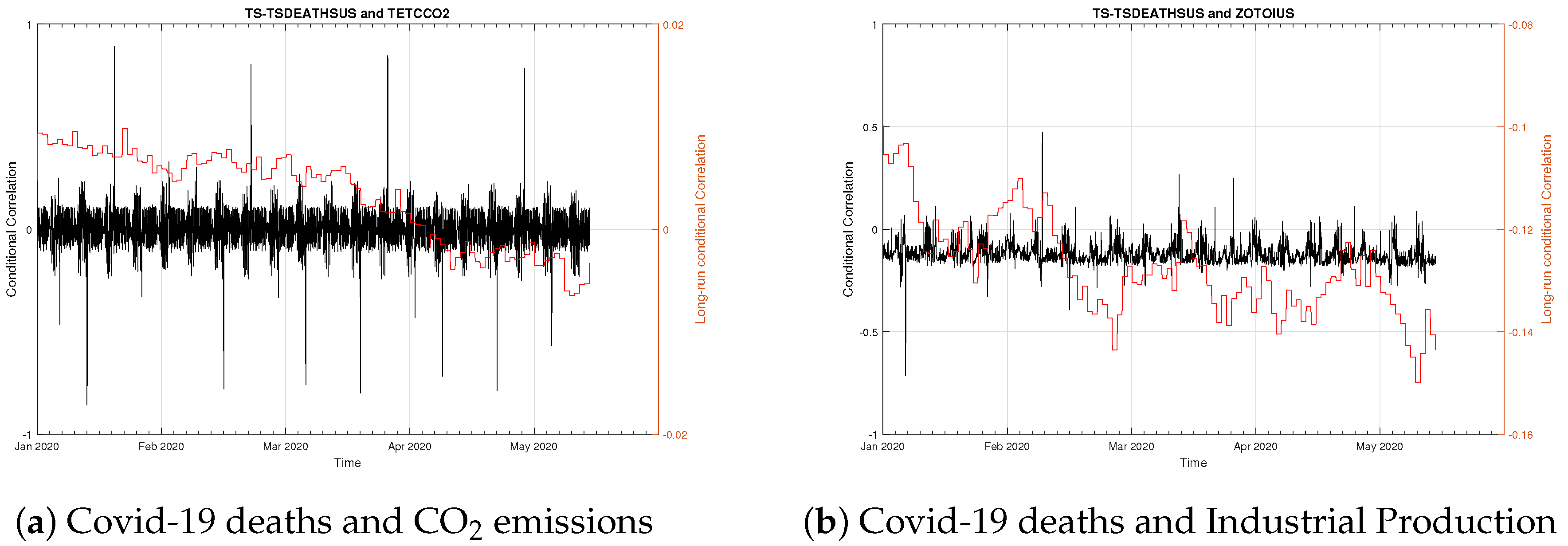
Looking at the variable, we estimate a statistically significant parameter , with a standard error of 2.91. When the number of deaths in the U.S. associated with the Coronavirus increases, the long-term macro-financial environment (and the associated fossil fuels CO emissions) decreases as a by-product.
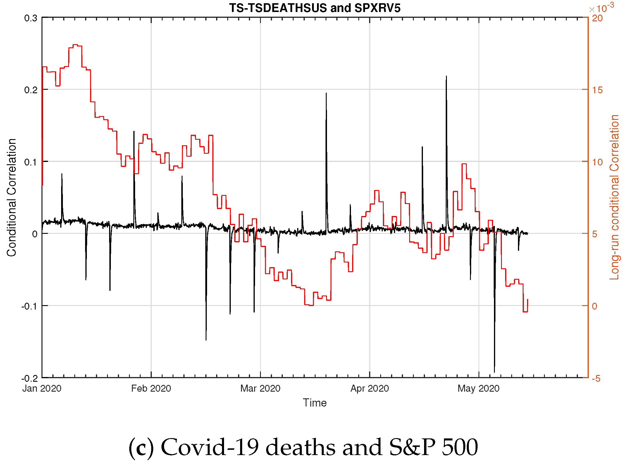
In Figure 5, macro-financial factors and CO emissions exhibit a decreasing long-run trend (in red) when interacting in the dynamic system of equations with COVID-19 deaths. In panel (c), we remark the volatility spikes (in black) agitating the stock market during the year 2020.
4.4. Introducing COVID-19 Recovered Cases
Last but not least, we turn to the number of COVID-19 recovered cases, which should be taken as a piece of “good” news for the U.S. economy. The estimation results are reproduced in Table 6.
Interestingly, the parameter estimate of for is statistically significant and positive, being equal to 1.85 with a standard error of 0.15. Hence, increases in the number of patients recovering from the COVID-19 should end the recession and re-start the economy (cyclical pattern).
All in all, we find that the COVID-19 variables are logically interacting with the set of macro-financial and CO emissions variables selected. The bad news (such as the multiplication of COVID-19 confirmed cases or deaths) degrades the business environment and production cycle. Recovery from the disease instills the hope of a better future "in the world after" the pandemic and the catching-up of economic growth.
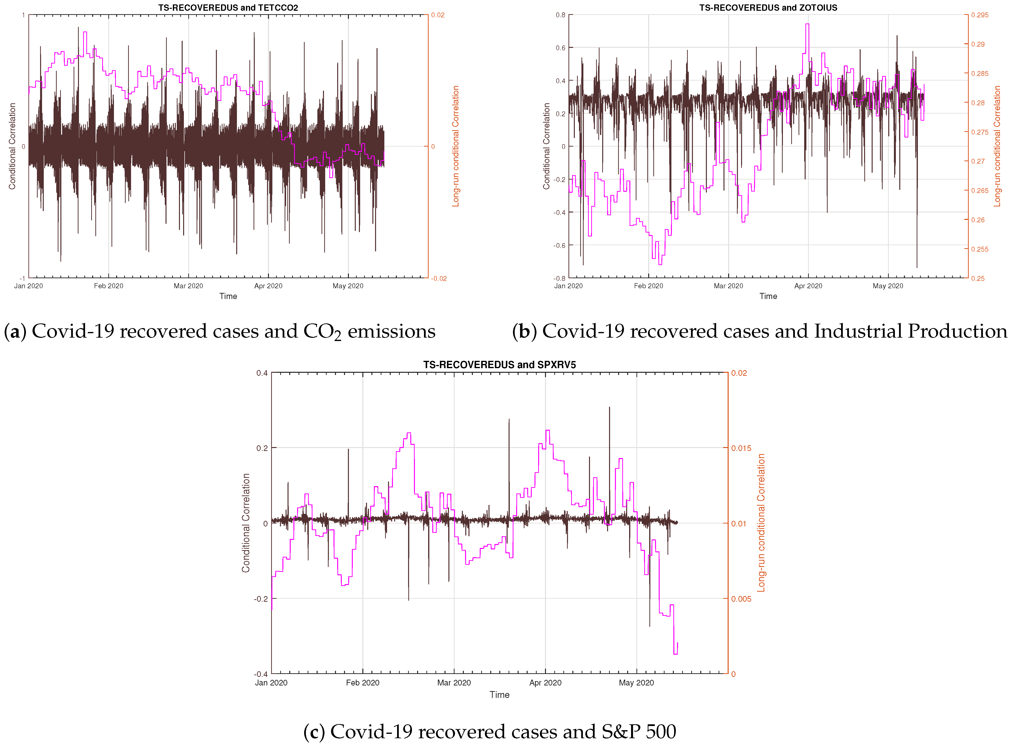
When looking at the panel (b) of Figure 6, we notice an increase in the long-run correlation (in pink color) between the COVID-19 recovered cases and industrial production, which might be subsumed as a piece of “good” news: when more people heal, the economy picks up.
However, we are not out of the economic recession cycle yet (not even by a small margin): in Figure 6, both long-run trends are decreasing when interacting COVID-19 recovered cases with either Total Fossil Fuel CO emissions or the S&P 500. Moreover, we again detect volatility spikes in panel (c) for the stock market (in brown color).
4.5. Sensitivity
In the present work, we have detailed estimation output from specifications, including the (3×) kinds of COVID-19 epidemiological cases, the Total Industrial Production Index (as a proxy of economic activity), the Total Fossil Fuels CO emissions, and the S&P 500 (as a proxy of the U.S. stock market). First, notice that the stability of parameters estimated for the variables , , and across Table 3, Table 4, Table 5 and Table 6 serves as a first kind of robustness check.
For further tests, we programmed a loop in order to estimate DCC-MIDAS with the remaining variables (i) (11 ×) macroeconomic indicators, (13 ×) manufacturing production indices, (four ×) price indexes, (five ×) miscellaneous and (ii) the (two ×) stock market indexes that are listed in Table 1 and Table 2. By browsing the log of results, we found that the paper’s main message is qualitatively unchanged.10 Namely, all of the parameter estimates keep their statistical significance, whilst the sign conforms to expected relationships.
5. Conclusions
The 45-day lock-down implemented during mid-March 2020 in most industrialized countries is expected to affect the real economy severely. In the meantime, it will alleviate part of the greenhouse gases’ burden that human activity induces on the environment. In this paper, we track both short- and long-run correlations in the Dynamic Conditional Correlation with Mixed Data Sampling (DCC-MIDAS) time-varying framework that enables data inputs from various (e.g., intra-daily, daily, and monthly) frequencies. The main variables of interest are the U.S. Total Fossil Fuel CO emissions, Total Industrial Production, and the S&P stock market. When we introduced the epidemiological cases of COVID-19, we uncovered two kinds of effects. On the one hand, the multiplication of COVID-19 confirmed cases and deaths seems to negatively influence the macro-financial environment (and associated CO emissions), as visible through MIDAS coefficients and long-run correlations. On the other hand, the increase in the number of patients healing from COVID-19 might be inferred as a good piece of news for the U.S. economy, being evident through the long-run correlation with industrial production. Other than that, we depict a recessionary macroeconomic outlook in the years to come, which is based on the identification of frequent spikes on stock markets against the pandemic background.
We may compare our results with previous studies in other fields, such as climate science. Zheng et al. (2020) use satellite observations together with bottom-up information to track the daily dynamics of CO emissions during the pandemic. The authors document that China’s CO emissions fell by 11.5% as compared to the same period in 2019. Le Quéré et al. (2020) estimate the decrease in CO emissions during forced confinements. According to them, the daily global CO emissions decreased by –17% by early April 2020 when compared with the mean 2019 levels. Liu et al. (2020) present the daily estimates of country-level CO emissions based on near-real-time activity data. The key result is an abrupt 8.8% decrease in global CO emissions in the first half of 2020 compared to the same period in 2019. These three scientific works relate to our estimates in the DCC-MIDAS model well. We quantified the time-varying correlations of CO emissions with either COVID-19 cases or COVID-19 deaths to sharply decrease by −15% to −30% as well.11
The present study is limited in its scope, to the extent that the data on CO emissions accessed only concern the start of the COVID-19 recession (aka, March 2020). Some economists (see, e.g., Diebold 2020) have already predicted that this sanitary crisis will turn into a “Pandemic Recession” in the years 2021–22 (for contagion effect to asset markets, see Chevallier 2020). Therefore, future research will be beneficial to assert the severity of the recession and the ultimate quantitative impact on CO emissions. Further studies in the fields of international production logistics and worldwide tourism, but not limited to them, would be promising areas to document this historical crisis better.
Funding
This research received no external funding.
Institutional Review Board Statement
Not applicable.
Informed Consent Statement
Not applicable.
Data Availability Statement
Publicly available datasets were analyzed in this study. This data can be found here: https://coronavirus.jhu.edu; https://www.eia.gov; and https://realized.oxford-man.ox.ac.uk.
Conflicts of Interest
The author declares no conflict of interest.
Appendix A
Setting the MIDAS Lags
The setting of the MIDAS lags is data-driven. Indeed, to accommodate various frequencies within the same methodological framework, the parameters , , and are not necessarily the same for all series (i.e., they differ depending on the monthly or daily frequency considered).
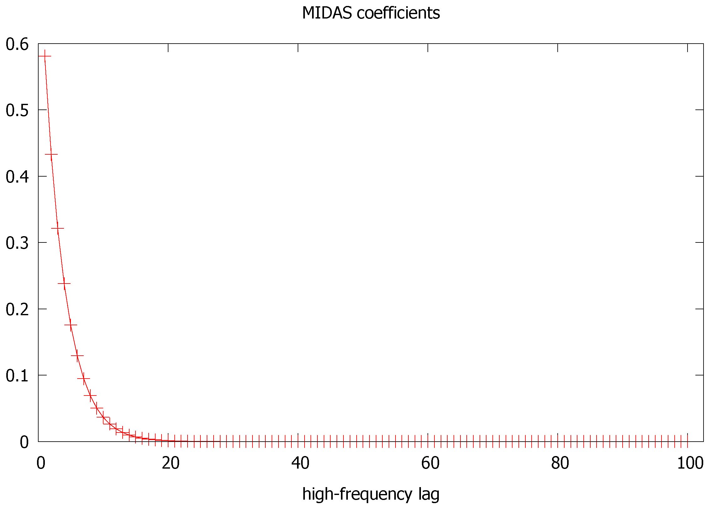
Ghysels et al. (2007) underline that most MIDAS regressors involve polynomials putting hardly any weight on longer lags. Engle et al. (2013) show that the optimal weights decay to 0 around thirty months of lags, regardless of the choice of t and length of MIDAS lag year.
This paper chooses 36 MIDAS lags for the conditional volatility process and 144 for the conditional correlation. This is similar to the original setting of Colacito et al. (2011) in their empirical application to stocks and bonds.
Figure A1.
MIDAS lags for the baseline specification.

An example of how this lag setting fares to the data is given in Figure A1 for the baseline specification. We notice that past 20 lags indeed, no further information is gained from the optimal weighting function. Hence, our setting of 36 lags for the conditional volatility process appears as a conservative choice.12
References
- Aatola, Piia, Markku Ollikainen, and Anne Toppinen. 2013. Price determination in the eu ets market: Theory and econometric analysis with market fundamentals. Energy Economics 36: 380–95. [Google Scholar] [CrossRef]
- Albulescu, Claudiu Tiberiu. 2020. COVID-19 and the united states financial markets’ volatility. Finance Research Letters, 101699. [Google Scholar] [CrossRef] [PubMed]
- Asgharian, Hossein, Charlotte Christiansen, and Ai Jun Hou. 2016. Macro-finance determinants of the long-run stock–bond correlation: The dcc-midas specification. Journal of Financial Econometrics 14: 617–42. [Google Scholar] [CrossRef]
- Azimli, Asil. 2020. The impact of covid-19 on the degree of dependence and structure of risk-return relationship: A quantile regression approach. Finance Research Letters 36: 101648. [Google Scholar] [CrossRef]
- Bai, Lan, Yu Wei, Guiwu Wei, Xiafei Li, and Songyun Zhang. 2020. Infectious disease pandemic and permanent volatility of international stock markets: A long-term perspective. Finance Research Letters, 101709. [Google Scholar] [CrossRef]
- Baig, Ahmed, Hassan A Butt, Omair Haroon, and Syed Aun R Rizvi. 2020. Deaths, panic, lockdowns and us equity markets: The case of covid-19 pandemic. Finance Research Letters, 101701. [Google Scholar] [CrossRef]
- Baker, Scott R., Nicholas Bloom, Steven J. Davis, Kyle Kost, Marco Sammon, and Tasaneeya Viratyosin. 2020. The unprecedented stock market reaction to covid-19. The Review of Asset Pricing Studies 10: 742–58. [Google Scholar] [CrossRef]
- Barndorff-Nielsen, Ole E, Peter Reinhard Hansen, Asger Lunde, and Neil Shephard. 2008. Designing realized kernels to measure the ex post variation of equity prices in the presence of noise. Econometrica 76: 1481–536. [Google Scholar]
- Carlsson-Szlezak, Philipp, Martin Reeves, and Paul Swartz. 2020. What coronavirus could mean for the global economy. Harvard Business Review 3: 1–10. [Google Scholar]
- Chevallier, Julien. 2011a. Evaluating the carbon-macroeconomy relationship: Evidence from threshold vector error-correction and markov-switching var models. Economic Modelling 28: 2634–56. [Google Scholar] [CrossRef]
- Chevallier, Julien. 2011b. A model of carbon price interactions with macroeconomic and energy dynamics. Energy Economics 33: 1295–1312. [Google Scholar] [CrossRef]
- Chevallier, Julien. 2012. Time-varying correlations in oil, gas and co2 prices: An application using bekk, ccc and dcc-mgarch models. Applied Economics 44: 4257–74. [Google Scholar] [CrossRef] [Green Version]
- Chevallier, Julien. 2020. COVID-19 pandemic and financial contagion. Journal of Risk and Financial Management 13: 309. [Google Scholar] [CrossRef]
- Colacito, Riccardo, Robert F Engle, and Eric Ghysels. 2011. A component model for dynamic correlations. Journal of Econometrics 164: 45–59. [Google Scholar] [CrossRef] [Green Version]
- Conrad, Christian, Karin Loch, and Daniel Rittler. 2014. On the macroeconomic determinants of long-term volatilities and correlations in us stock and crude oil markets. Journal of Empirical Finance 29: 26–40. [Google Scholar] [CrossRef]
- Diebold, Francis X. 2020. Real Time Economic Activity: Exiting the Great Recession and Entering the Pandemic Recession. IAAE Webinar Series; New York: International Association for Applied Econometrics. [Google Scholar]
- Engle, Robert F, Eric Ghysels, and Bumjean Sohn. 2013. Stock market volatility and macroeconomic fundamentals. Review of Economics and Statistics 95: 776–97. [Google Scholar] [CrossRef]
- Engle, Robert F, and Kevin Sheppard. 2001. Theoretical and empirical properties of dynamic conditional correlation multivariate garch. In National Bureau of Economic Research. Technical Report. Cambridge: NBER. [Google Scholar]
- Fell, Harrison. 2010. Eu-ets and nordic electricity: A cvar analysis. The Energy Journal 31: 1–17. [Google Scholar] [CrossRef]
- Gharib, Cheima, Salma Mefteh-Wali, and Sami Ben Jabeur. 2020. The bubble contagion effect of covid-19 outbreak: Evidence from crude oil and gold markets. Finance Research Letters, 101703. [Google Scholar] [CrossRef]
- Ghysels, Eric, Pedro Santa-Clara, and Rossen Valkanov. 2004. The Midas Touch: Mixed Data Sampling Regressions. Chapel Hill: University of North Carolina and UCLA. [Google Scholar]
- Ghysels, Eric, Arthur Sinko, and Rossen Valkanov. 2007. Midas regressions: Further results and new directions. Econometric Reviews 26: 53–90. [Google Scholar] [CrossRef]
- Gómez-Puig, Marta, and Simón Sosvilla-Rivero. 2016. Causes and hazards of the euro area sovereign debt crisis: Pure and fundamentals-based contagion. Economic Modelling 56: 133–47. [Google Scholar] [CrossRef] [Green Version]
- Gruppe, Mario, Tobias Basse, Meik Friedrich, and Carsten Lange. 2017. Interest rate convergence, sovereign credit risk and the european debt crisis: A survey. The Journal of Risk Finance 18: 432–42. [Google Scholar] [CrossRef]
- Hintermann, Beat. 2010. Allowance price drivers in the first phase of the eu ets. Journal of Environmental Economics and Management 59: 43–56. [Google Scholar] [CrossRef] [Green Version]
- Kamin, Steven B, and Laurie Pounder DeMarco. 2012. How did a domestic housing slump turn into a global financial crisis? Journal of International Money and Finance 31: 10–41. [Google Scholar] [CrossRef] [Green Version]
- Le Quéré, Corinne, Robert B. Jackson, Matthew W. Jones, Adam J. P. Smith, Sam Abernethy, Robbie M. Andrew, Anthony J. De-Gol, David R. Willis, Yuli Shan, Josep G. Canadell, and et al. 2020. Temporary reduction in daily global co2 emissions during the covid-19 forced confinement. Nature Climate Change 10: 1–7. [Google Scholar] [CrossRef]
- Liu, Zhu, Philippe Ciais, Zhu Deng, Ruixue Lei, Steven J. Davis, Sha Feng, Bo Zheng, Duo Cui, Zhu Xinyu, Guo Biqing, and et al. 2020. Near-real-time monitoring of global co2 emissions reveals the effects of the covid-19 pandemic. Nature Communications 11: 1–12. [Google Scholar] [CrossRef]
- Lutz, Benjamin Johannes, Uta Pigorsch, and Waldemar Rotfuß. 2013. Nonlinearity in cap-and-trade systems: The eua price and its fundamentals. Energy Economics 40: 222–32. [Google Scholar] [CrossRef] [Green Version]
- Lyócsa, Štefan, and Peter Molnár. 2020. Stock market oscillations during the corona crash: The role of fear and uncertainty. Finance Research Letters 36: 101707. [Google Scholar] [CrossRef]
- Mazur, Mieszko, Man Dang, and Miguel Vega. 2020. COVID-19 and the march 2020 stock market crash. evidence from s&p1500. Finance Research Letters, 101690. [Google Scholar] [CrossRef]
- Melvin, Michael, and Mark P Taylor. 2009. The global financial crisis: Causes, threats and opportunities. introduction and overview. Journal of International Money and Finance 28: 1243–1245. [Google Scholar] [CrossRef]
- Moro, Beniamino. 2014. Lessons from the european economic and financial great crisis: A survey. European Journal of Political Economy 34: S9–S24. [Google Scholar] [CrossRef]
- National Academies of Sciences, Engineering, Medicine. 2020. Framework for Equitable Allocation of COVID-19 Vaccine. Washington: National Academies Press. [Google Scholar]
- Papadamou, Stephanos, Athanasios P. Fassas, Dimitris Kenourgios, and Dimitrios Dimitriou. 2020. Flight-to-quality between global stock and bond markets in the covid era. Finance Research Letters, 101852. [Google Scholar] [CrossRef]
- Rizwan, Muhammad Suhail, Ghufran Ahmad, and Dawood Ashraf. 2020. Systemic risk: The impact of covid-19. Finance Research Letters, 101682. [Google Scholar] [CrossRef] [PubMed]
- Sohrabi, Catrin, Zaid Alsafi, Niamh O’Neill, Mehdi Khan, Ahmed Kerwan, Ahmed Al-Jabir, Christos Iosifidis, and Riaz Agha. 2020. World health organization declares global emergency: A review of the 2019 novel coronavirus (covid-19). International Journal of Surgery. [Google Scholar] [CrossRef]
- Topcu, Mert, and Omer Serkan Gulal. 2020. The impact of covid-19 on emerging stock markets. Finance Research Letters 36: 101691. [Google Scholar] [CrossRef]
- Wegener, Christoph, Robinson Kruse, and Tobias Basse. 2019. The walking debt crisis. Journal of Economic Behavior & Organization 157: 382–402. [Google Scholar]
- Xu, Qifa, Lu Chen, Cuixia Jiang, and Jing Yuan. 2018. Measuring systemic risk of the banking industry in china: A dcc-midas-t approach. Pacific-Basin Finance Journal 51: 13–31. [Google Scholar] [CrossRef]
- Zheng, Bo, Guannan Geng, Philippe Ciais, Steven J. Davis, Randall V. Martin, Jun Meng, Nana Wu, Frederic Chevallier, Gregoire Broquet, Folkert Boersma, and et al. 2020. Satellite-based estimates of decline and rebound in china’s co2 emissions during covid-19 pandemic. Science Advances, 6. [Google Scholar] [CrossRef]
| 1 | Academically, it is interesting to investigate whether the two crisis events are connected to each other. As argued by Gómez-Puig and Sosvilla-Rivero (2016), the European sovereign debt crisis is preceded by contagion episodes with causal links that stem from the Global Financial Crisis’s outburst. Wegener et al. (2019) challenge the view that the arising sovereign credit risk in the EMU has been triggered by the U.S. subprime crunch. On the contrary, they conclude that the severe fiscal problems in peripheral countries are homemade, rather than imported from the U.S. Thus, no definitive conclusion seems to be reached based on quantitative analysis. |
| 2 | Such as the excessive dependence on short-term funding; or vicious cycles of mark-to-market losses driving fire sales of mortgage-backed securities. |
| 3 | |
| 4 | |
| 5 | |
| 6 | Precisely, the EIA’s Table 9a accessed from https://www.eia.gov/totalenergy/data/browser/. |
| 7 | See Barndorff-Nielsen et al. (2008) for the theory. |
| 8 | Upon reasonable request, we can transmit (unformatted) unit root tests in order to show that, thus transformed, the series are indeed . |
| 9 | To save space, conditional variances not shown here and they can be transmitted upon request to the interested reader. |
| 10 | Upon a reasonable request, we can transmit (unformatted) logs of DCC-MIDAS estimates. The computational burden induced by the loop (e.g., combinations) can create memory usage bottlenecks on lower-end computers. |
| 11 | |
| 12 | Upon request, a similar analysis can be produced for the 144 lag settings of the conditional correlation. It is not shown for brevity. |
Figure 1.
Monthly U.S. Total Fossil Fuel CO emissions (top), Monthly U.S. Industrial Production Index Seasonally Adjusted (middle) and S&P 500 Index (bottom) daily close. Note: CO emissions are sourced from U.S. Energy Information Administration. Industrial production and S&P 500 are sourced from the Federal Reserve Bank of St. Louis.

Figure 2.
U.S. COVID-19 confirmed cases (top), deaths (middle), and recovered cases (bottom) extracted from the Johns Hopkins Repository on 5 May 2020.
Figure 2.
U.S. COVID-19 confirmed cases (top), deaths (middle), and recovered cases (bottom) extracted from the Johns Hopkins Repository on 5 May 2020.

Figure 3.
Conditional correlation (blue) and Long-run conditional correlation (green) for the baseline specification.
Figure 3.
Conditional correlation (blue) and Long-run conditional correlation (green) for the baseline specification.

Figure 4.
Conditional correlation (blue) and Long-run conditional correlation (orange) when introducing COVID-19 confirmed cases in the baseline specification.
Figure 4.
Conditional correlation (blue) and Long-run conditional correlation (orange) when introducing COVID-19 confirmed cases in the baseline specification.

Figure 5.
Conditional correlation (black) and Long-run conditional correlation (red) when introducing COVID-19 deaths in the baseline specification.
Figure 5.
Conditional correlation (black) and Long-run conditional correlation (red) when introducing COVID-19 deaths in the baseline specification.


Figure 6.
Conditional correlation (black) and Long-run conditional correlation (red) when introducing COVID-19 recovered cases in the baseline specification.
Figure 6.
Conditional correlation (black) and Long-run conditional correlation (red) when introducing COVID-19 recovered cases in the baseline specification.


Table 1.
U.S. EIA database on Macroeconomic indicators and CO emissions.
| Macroeconomic | |
| Real Gross Domestic Product | |
| Real Personal Consumption Expenditures | |
| Real Private Fixed Investment | |
| Business Inventory Change | |
| Real Government Expenditures | |
| Real Exports of Goods & Services | |
| Real Imports of Goods & Services | |
| Real Disposable Personal Income | |
| Non-Farm Employment | |
| Civilian Unemployment Rate | |
| Housing Starts | |
| Manufacturing Production Indices | |
| Total Industrial Production Index | |
| Manufacturing Production Index | |
| Food Production Index (NAICS 311) | |
| Paper Production Index (NAICS 322) | |
| Petroleum and Coal Products Production Index (NAICS 324) | |
| Chemicals Production Index (NAICS 325) | |
| Resins and Synthetic Products Production Index (NAICS 3252) | |
| Agricultural Chemicals Production Index | |
| Nonmetallic Mineral Products Production Index | |
| Primary Metals Production Index (NAICS 311) | |
| Coal-weighted Manufacturing Production Index | |
| Distillate-weighted Manufacturing Production Index | |
| Electricity-weighted Manufacturing Production Index | |
| Natural Gas-weighted Manufacturing Production Index | |
| Price Indexes | |
| Consumer Price Index (all urban consumers) | |
| Producer Price Index: All Commodities | |
| Producer Price Index: Petroleum | |
| GDP Implicit Price Deflator | |
| Miscellaneous | |
| Vehicle Miles Traveled | |
| Air Travel Capacity | |
| Aircraft Utilization | |
| Airline Ticket Price Index | |
| Raw Steel Production | |
| Carbon Dioxide (CO) Emissions | |
| Petroleum CO Emissions | |
| Natural Gas CO Emissions | |
| Coal CO Emissions | |
| Total Fossil Fuels CO Emissions |
Table 2.
Oxford-Man’s Realized Library: U.S. stock markets.
| Symbol | Name | Earliest Available | Latest Available |
|---|---|---|---|
| .DJI | Dow Jones Industrial Average | 3 January 2000 | 8 May 2020 |
| .IXIC | Nasdaq 100 | 3 January 2000 | 8 May 2020 |
| .SPX | S&P 500 Index | 3 January 2000 | 8 May 2020 |
Table 3.
Dynamic Conditional Correlation with Mixed Data Sampling (DCC-MIDAS) estimates for the baseline specification including Total Fossil Fuels CO emissions, Total Industrial Production Index, and S&P 500 Index.
Table 3.
Dynamic Conditional Correlation with Mixed Data Sampling (DCC-MIDAS) estimates for the baseline specification including Total Fossil Fuels CO emissions, Total Industrial Production Index, and S&P 500 Index.
| m | ||||||
|---|---|---|---|---|---|---|
| TETCCO2 | 0.2797 *** | 0.0469 *** | 0.5986 *** | 0.1000 *** | 5.7068 *** | 7.7439 *** |
| (0.0001) | (0.0002) | (0.0013) | (0.0003) | (0.0005) | (0.0001) | |
| ZOTOIUS | −0.1181 | 0.0142 *** | 0.9858 *** | 0.1368 | 1.001 0 | 32.3250 *** |
| (0.1101) | (0.0004) | (0.0004) | (9.9118 ) | (13.4850) | (3.6880) | |
| SPX-RV5 | 0.0015 | 0.2344 *** | 0.0556 | 0.1939 *** | 6.4697 *** | 0.3568 *** |
| (0.0090) | (0.0245) | (0.0574) | (0.0142) | (2.0287) | (0.0678) | |
| a | b | |||||
| DCC-MIDAS | 0.0171 | 0.8000 | 1.001 *** | |||
| (0.0204) | (0.6090 ) | (0.2088) | ||||
| Logarithmic likelihood: | −6430.57 | |||||
| Akaike info criterion: | 12,867.1 | |||||
| Bayesian info criterion: | 12,886.7 | |||||
| Sample size: | 5103 |
Note: *** indicates statistical significance at the 1% level. The sample covers 3 January 2020 to 8 May 2020. TETCCO2 is the Total Fossil Fuels CO emissions. ZOTOIUS is the Total Industrial Production Index. SPX-RV5 is the five-minute Realized Volatility of the S&P 500 Index. Equations (1)–(5) detail the conditional correlation. The conditional volatility is specified as a GARCH-MIDAS: , with the daily time scale, and the classic ARCH and GARCH parameters, the monthly MIDAS component for the time scale that changes every days as a weighted sum of lags, and the main MIDAS parameter of various lag polynomials for parsimony.
Table 4.
Dynamic Conditional Correlation with Mixed Data Sampling (DCC-MIDAS) estimates when introducing COVID-19 confirmed cases to the baseline that is composed of Total Fossil Fuels CO emissions, Total Industrial Production Index, and S&P 500 Index.
Table 4.
Dynamic Conditional Correlation with Mixed Data Sampling (DCC-MIDAS) estimates when introducing COVID-19 confirmed cases to the baseline that is composed of Total Fossil Fuels CO emissions, Total Industrial Production Index, and S&P 500 Index.
| m | ||||||
|---|---|---|---|---|---|---|
| TS-CONFIRMED-US | 12969.7920 | 0.9999 *** | 0.0001 *** | −28.4962 *** | 1.0830 *** | 0.0100 *** |
| (12085) | (0.3189) | (0.0001) | (6.8426) | (0.1688) | (0.0005) | |
| TETCCO2 | 0.2796 *** | 0.0468 *** | 0.5980 *** | 0.1000 *** | 5.7067 *** | 7.7438 *** |
| (0.0001) | (0.0001) | (0.0001) | (0.0001) | (0.0001) | (0.0001) | |
| ZOTOIUS | −0.1180 | 0.0141*** | 0.9857 *** | 0.1368 | 1.001 | 32.3246 *** |
| (0.1103) | (0.0004) | (0.0004) | (9.9118) | (13.4850) | (3.688) | |
| SPX-RV5 | 0.0015 | 0.2344 *** | 0.0556 | 0.1938 *** | 6.4696 *** | 0.3567 *** |
| (0.0090) | (0.0245) | (0.0574) | (0.0142) | (2.0287) | (0.0678) | |
| a | b | |||||
| DCC-MIDAS | 0.0178 | 0.6012 | 1.001 *** | |||
| (0.0291) | (0.8847) | (0.4317) | ||||
| Logarithmic likelihood: | −6334.08 | |||||
| Akaike info criterion: | 12,674.2 | |||||
| Bayesian info criterion: | 12,693.8 | |||||
| Adjusted sample size: | 1503 |
Note: *** indicates statistical significance at the 1% level. The sample covers 22 January 2020 to 8 May 2020. TS-CONFIRMED-US is the number of COVID-19 confirmed cases in the USA. TETCCO2 is the Total Fossil Fuels CO emissions. ZOTOIUS is the Total Industrial Production Index. SPX-RV5 is the 5-minute Realized Volatility of the S&P 500 Index. Equations (1)–(5) detail the conditional correlation. The conditional volatility is specified as a GARCH-MIDAS: , with the daily time scale, and the classic ARCH and GARCH parameters, the monthly MIDAS component for the time scale that changes every days as a weighted sum of lags, and the main MIDAS parameter of various lag polynomials for parsimony.
Table 5.
Dynamic Conditional Correlation with Mixed Data Sampling (DCC-MIDAS) estimates when introducing COVID-19 deaths to the baseline composed of Total Fossil Fuels CO emissions, Total Industrial Production Index, and S&P 500 Index.
Table 5.
Dynamic Conditional Correlation with Mixed Data Sampling (DCC-MIDAS) estimates when introducing COVID-19 deaths to the baseline composed of Total Fossil Fuels CO emissions, Total Industrial Production Index, and S&P 500 Index.
| m | ||||||
|---|---|---|---|---|---|---|
| TS-DEATHS-US | 760.71748 | 0.9999 *** | 0.0001 *** | −46.2930 *** | 1.0836 *** | 0.0100 *** |
| (633.73) | (0.3178) | (0.0001) | (2.9142) | (0.1697) | (0.0005) | |
| TETCCO2 | 0.2799 *** | 0.0468 *** | 0.5986 *** | 0.1000 *** | 5.7068 *** | 7.7439 *** |
| (0.0001) | (0.0001) | (0.0001) | (0.0001) | (0.0001) | (0.0001) | |
| ZOTOIUS | −0.1181 | 0.0146 *** | 0.9859 *** | 0.1366 | 1.0010 | 32.3250 *** |
| (0.1137) | (0.0004) | (0.0004) | (9.9118) | (13.4850) | (3.6880) | |
| SPX-RV5 | 0.0016 | 0.2343 *** | 0.0557 | 0.1939 *** | 6.4697 *** | 0.3577 *** |
| (0.0091) | (0.0246) | (0.0577) | (0.0141) | (2.0287) | (0.0688) | |
| a | b | |||||
| DCC-MIDAS | 0.0163 | 0.6430 | 1.001 *** | |||
| (0.0272) | (0.8376) | (0.4335) | ||||
| Logarithmic likelihood: | −6334.93 | |||||
| Akaike info criterion: | 12,677 | |||||
| Bayesian info criterion: | 12,696.6 | |||||
| Adjusted sample size: | 1503 |
Note: *** indicates statistical significance at the 1% level. The sample covers 22 January 2020 to 8 May 2020. TS-DEATHS-US is the number of COVID-19 deaths in the USA. TETCCO2 is the Total Fossil Fuels CO emissions. ZOTOIUS is the Total Industrial Production Index. SPX-RV5 is the 5-min. Realized Volatility of the S&P 500 Index. Equations (1)–(5) detail the conditional correlation. The conditional volatility is specified as a GARCH-MIDAS: , with the daily time scale, and the classic ARCH and GARCH parameters, the monthly MIDAS component for the time scale that changes every days as a weighted sum of lags, and the main MIDAS parameter of various lag polynomials for parsimony.
Table 6.
Dynamic Conditional Correlation with Mixed Data Sampling (DCC-MIDAS) estimates when introducing COVID-19 recovered cases to the baseline composed of Total Fossil Fuels CO emissions, Total Industrial Production Index, and S&P 500 Index.
Table 6.
Dynamic Conditional Correlation with Mixed Data Sampling (DCC-MIDAS) estimates when introducing COVID-19 recovered cases to the baseline composed of Total Fossil Fuels CO emissions, Total Industrial Production Index, and S&P 500 Index.
| m | ||||||
|---|---|---|---|---|---|---|
| TS-RECOVERED-US | −2567.0739 ** | 0.6144 *** | 0.3778 *** | 1.8502 *** | 1.0876 *** | 0.0100 |
| (1041.40) | (0.0354) | (0.0328) | (0.1576) | (0.2205) | (0.0006) | |
| TETCCO2 | 0.2769 *** | 0.0488 *** | 0.5980 *** | 0.1000 *** | 5.7068 *** | 7.7439 *** |
| (0.0001) | (0.0001) | (0.0001) | (0.0001) | (0.0001) | (0.0001) | |
| ZOTOIUS | −0.1189 | 0.0147 *** | 0.9857 *** | 0.1368 | 1.0010 | 32.3250 *** |
| (0.1137) | (0.0004) | (0.0004) | (9.9118) | (13.4850) | (3.6880) | |
| SPX-RV5 | 0.0015 | 0.2344 *** | 0.0557 | 0.1938 *** | 6.4697 *** | 0.3568 *** |
| (0.0090) | (0.0245) | (0.0574) | (0.0142) | (2.0287) | (0.0675) | |
| a | b | |||||
| DCC-MIDAS | 0.0278 | 0.6170 *** | 1.001 *** | |||
| (0.0383) | (0.0813 | (0.3917) | ||||
| Logarithmic likelihood: | −6492.48 | |||||
| Akaike info criterion: | 12,991 | |||||
| Bayesian info criterion: | 13,010.6 | |||||
| Adjusted sample size: | 1503 |
Note: *** (**) indicates statistical significance at the 1% (5%) level. The sample covers 22 January 2020 to 8 May 2020. TS-RECOVEREDUS is the number of COVID-19 recovered cases in the USA. TETCCO2 is the Total Fossil Fuels CO emissions. ZOTOIUS is the Total Industrial Production Index. SPX-RV5 is the 5-minute Realized Volatility of the S&P 500 Index. Equations (1)–(5) detail the conditional correlation. The conditional volatility is specified as a GARCH-MIDAS: , with the daily time scale, and the classic ARCH and GARCH parameters, the monthly MIDAS component for the time scale that changes every days as a weighted sum of lags, and the main MIDAS parameter of various lag polynomials for parsimony.
Publisher’s Note: MDPI stays neutral with regard to jurisdictional claims in published maps and institutional affiliations. |
© 2020 by the author. Licensee MDPI, Basel, Switzerland. This article is an open access article distributed under the terms and conditions of the Creative Commons Attribution (CC BY) license (http://creativecommons.org/licenses/by/4.0/).
Share and Cite
MDPI and ACS Style
Chevallier, J. COVID-19 Outbreak and CO2 Emissions: Macro-Financial Linkages. J. Risk Financial Manag. 2021, 14, 12. https://doi.org/10.3390/jrfm14010012
AMA Style
Chevallier J. COVID-19 Outbreak and CO2 Emissions: Macro-Financial Linkages. Journal of Risk and Financial Management. 2021; 14(1):12. https://doi.org/10.3390/jrfm14010012
Chicago/Turabian StyleChevallier, Julien. 2021. "COVID-19 Outbreak and CO2 Emissions: Macro-Financial Linkages" Journal of Risk and Financial Management 14, no. 1: 12. https://doi.org/10.3390/jrfm14010012