Analyzing the Data of COVID-19 with Quasi-Distribution Fitting Based on Piecewise B-Spline Curves

Abstract

Facing the worldwide coronavirus disease 2019 (COVID-19) pandemic, a new fitting method (QDF, quasi-distribution fitting) which can be used to analyze the data of COVID-19 is developed based on piecewise quasi-uniform B-spline curves. For any given country or district, it simulates the distribution histogram data which is made from the daily confirmed cases (or the other data including daily recovery cases and daily fatality cases) of COVID-19 with piecewise quasi-uniform B-spline curves. After using the area normalization method, the fitting curves could be regarded as a kind of probability density function (PDF): its mathematical expectation and the variance could be used to analyze the situation of the coronavirus pandemic. Numerical experiments based on the data of certain countries have indicated that the QDF method demonstrates the intrinsic characteristics of COVID-19 data of a given country or district, and because the interval of data used in this paper is over one year (500 days), it reveals the fact that after the multi-wave transmission of the coronavirus, the case fatality rate has obviously declined. These results show that the QDF method is effective and feasible as an appraisal method.

1. Introduction

In late December 2019, cases of pneumonia with an unknown etiology were reported in the city of Wuhan, China [1]. The causative agent, identified as the betacoronavirus SARS-CoV-2, is closely related to SARS-CoV, which was responsible [2] for the outbreak of SARS between 2002 and 2004. SARS-CoV-2 caused a sizable epidemic of COVID-19 in China, then spread globally and was declared a pandemic in March 2020 [3]. There have been many research articles about this pandemic, examining the plague from different angles. Some compared its pathogenesis with that of Middle East respiratory syndrome (MERS) and SARS [4] and how COVID-19 pneumonia compromises the distal lung’s ability to perform essential respiratory functions [5], while others detailed the virological analysis of cases of COVID-19 that provide proof of active virus replication in tissues of the upper respiratory tract [6]. Some discussed the COVID-19-related mortality among different ages [7], genders [8], or races [9], and also shed light on the frequency of asymptomatic SARS-CoV-2 infection [10]. There were also a lot of research works focusing on building mathematical models to simulate the spread of SARS-CoV-2, such as the metapopulation susceptible-exposed-infectious-removed (SEIR) model, which integrated fine-grained, dynamic mobility networks simulating the spread of COVID-19 in ten of the largest US metropolitan areas [11], and the full-spectrum dynamics model, which reconstructed the transmission mode of COVID-19 in Wuhan between 1 January and 8 March 2020 [12]. The analyses of data show how anti-contagion polices have significantly and substantially slowed the growth of COVID-19 infections [13], and the major non-pharmaceutical interventions—and lockdowns in particular—have had a large effect on reducing transmission [14] in the same way. One research group studied the relationship between socio-economic factors and the COVID-19 pandemic in Germany: analyzing both infections and fatalities showed that the population of poorer and more socially deprived districts is not necessarily more likely to get infected with SARS-CoV-2, but combines an average infection rate with a higher than average death rate [15]. Apart from these social problems caused by COVID-19, it has also changed people’s everyday life praxis during restriction measures [16].

Estimating the size of the coronavirus disease 2019 (COVID-19) pandemic is made challenging by inconsistencies in the available data [17], so it is very important to analyze the COVID-19 data of a given country or district, including the number of daily confirmed cases, daily recovery cases, and daily fatality cases. In this paper, we use a quasi-distribution fitting method based on piecewise quasi-uniform B-spline curves to investigate the consistency of infection and therapy patterns across multiple countries. It is established by fitting the distribution histogram data made from the COVID-19 data of a given country or district with piecewise quasi-uniform B-spline curves; then using the area normalization process, the fitting curves can be regarded as a kind of probability density function (PDF) of the data, then the mathematical expectation and the variance can be calculated as the evaluation result.

2. Theoretical Considerations

In computer-aided geometric design, the B-spline form is widely used in representing a polynomial curve. B-spline curves have optimal shape preserving properties, and a B-spline curve of order $n$ is evaluated by the de Casteljau algorithm with a computational cost of $O\left(n^2\right)$ elementary operations [18]. However, B-spline curves also have shortcomings; they are a kind of curve whose control polygon is not combined with the curve itself at the endpoints, which means by changing just one control point the majority of the curve will be changed. Thus, in this paper we will use piecewise quasi-uniform B-spline curves to fulfill the fitting works.

2.1. Histogram Distribution

Because of the delay in epidemiology statistics systems of different countries or districts, we needed to precondition the data before the fitting process.

Table 1. Daily new cases of different countries in five days.

Finland		France		Korea		Ecuador
11/4/2020	293	7/2/2020	659	1/15/2021	513	7/13/2020	589
11/5/2020	189	7/3/2020	582	1/16/2021	1099	7/14/2020	0
11/6/2020	266	7/4/2020	0	1/17/2021	0	7/15/2020	1870
11/7/2020	0	7/5/2020	0	1/18/2021	389	7/16/2020	1036
11/8/2020	412	7/6/2020	1375	1/19/2021	386	7/17/2020	1079

shows five daily confirmed cases data of four countries: from the first column, we can see that the daily confirmed cases in Finland from 4 November 2020 to 6 November 2020 was around 200 per day, but on 7 November 2020 it was down to zero, and then was back to 412 on 8 November 2020, almost twice that of the previous data.

The most probable explanation is that the data of the daily confirmed cases from 7 November 2020 were delayed and then combined with the data of the following day. The same happened in the data from France, Korea, and Ecuador; the simple way to avoid this issue was to use adjacent average data instead of the original data. In this paper, we use 7-day moving average data to fulfill our research plan, which means in order to get the 7-day moving average data, we needed an extra three days of data on both sides of the data interval. For example, the data interval for Italy we used in this paper was from 21 February 2020 to 4 July 2021, containing 500 days of data, but the actual data we used were from 18 February 2020 to 7 July 2021. For a given country or district, $D_k$ denotes the 7-day moving average of the number of daily confirmed cases on day $k$; letting $N$ be the data interval (in this paper $N=500$), for Italy, $D_1$ is 7-day moving average of the daily confirmed cases of February 21st, which is the average of the daily confirmed cases from 18 February 2020 to 24 February 2020.

$$\mathrm{Assume}{D}_{\sigma }={{\displaystyle \sum }}_{i=1}^N{D}_i,\mathrm{let}{f}_k^D=\frac{D_k}{D_{\sigma }},\mathrm{then}\mathrm{we}\mathrm{have} {{\displaystyle \sum }}_{k=1}^N{f}_k^D=1$$

This means $f_k^D$ can be regarded as a kind of probability distribution, which can be called a histogram distribution.

Table 2. Beginning date and ending date of different countries’ COVID-19 data.

Country	Beginning Date	Ending Date	Country	Beginning Date	Ending Date
Austria	3/01/2020	7/13/2021	Brazil	3/06/2020	7/18/2021
Canada	2/28/2020	7/11/2021	Chile	3/04/2020	7/16/2021
The US	2/29/2020	7/12/2021	Denmark	3/02/2020	7/14/2021
France	2/26/2020	7/09/2021	Germany	2/29/2020	7/12/2021
India	3/02/2020	7/14/2021	Iran	2/19/2020	7/02/2021
Israel	3/06/2020	7/18/2021	Italy	2/21/2020	7/04/2021
Japan	1/29/2020	6/11/2021	Korea	2/17/2020	6/30/2021
Lebanon	2/26/2020	7/09/2021	The Philippines	3/07/2020	7/19/2021
Poland	3/04/2020	7/16/2021	Portugal	2/24/2020	7/07/2021

show the beginning date and the ending date of the COVID-19 data from the countries used in our fitting process.

2.2. Piecewise Quasi-Uniform B-Spline Curve

For those histogram distribution data $f_k^D$, they can be simulated with a function $P\left(x\right)$, which has the properties of a probability density function (PDF). Thus, the histogram distribution data $f_k^D$ can be analyzed from the respective probability theory. In this paper, we fit $f_k^D$ with piecewise quasi-uniform B-spline curve, which is more flexible in curve modeling. A piecewise quasi-uniform B-spine curve is a kind of parameter curve (here the parameter is denoted as $t\in \left[0,1\right]$) that is obtained from a uniform B-spline curve. First, we give the base functions of five-order quasi-uniform B-spline curves defined on interval $\left[0,1\right]$, whose node vector divides $\left[0,1\right]$ into ten subintervals evenly, denoting them as ${\tilde{N}}_i,i=0,1,\cdots 14$. The concrete expression of those base functions ${\tilde{N}}_i$ can be found in Appendix A. Second, we define the base functions of the piecewise quasi-uniform B-spline as follows:

$$\begin{array}{l}{N}_i\left(t\right)=\{\begin{array}{c}{\tilde{N}}_i\left(\frac{t}{\omega }\right)t\in 0,\omega )\\ 0 t\in \left[\omega ,1\right]\end{array}i=0,1,\cdots 13,N_{14}\left(t\right)=\{\begin{array}{c}{\tilde{N}}_{14}\left(\frac{t}{\omega }\right)t\in 0,\omega )\\ {\tilde{N}}_0\left(\frac{1-t}{1-\omega }\right)t\in \left[\omega ,1\right]\end{array},\\ N_i\left(t\right)=\{\begin{array}{c}0 t\in 0,\omega )\\ {\tilde{N}}_{i-14}\left(\frac{1-t}{1-\omega }\right)t\in \left[\omega ,1\right]\end{array}i=15,\cdots ,28,\mathrm{where}\omega \in \left(0,1\right)\mathrm{is}\mathrm{the}\mathrm{segmentation}\mathrm{point}.\end{array}$$

Assuming$C_i,i=0,1,\cdots 28$are the points in a two-dimensional plane, then the definition of a quintic piecewise quasi-uniform B-spline curve is as follows:

$$B\left(t\right)={\displaystyle \sum }_{i=0}^{28}{N}_i\left(t\right)C_{i}t\in \left[0,1\right]$$

(1)

where $C_i$ are the control points of the curve defined by Equation (1).

3. Fitting Process

Given a histogram distribution data $f_k^D$, we need to find the corresponding quintic piecewise quasi-uniform B-spline curve $B\left(t\right)={{\displaystyle \sum }}_{i=0}^{28}{N}_i\left(t\right)C_i$ to fit it. The most important part is to calculate the unknown control points $C_i$.

3.1. Least Square Approximation Method

In this paper, we use the least square approximation to deal with this problem. First, parameterize the data $f_k^D$ by the cumulative chord length parameterization method to match a parameter $t_k$ for every $f_k^D$, thus obtaining a parametric sequence $0=t_1<\cdots t_k<\cdots <t_N=1$. Second, assume ${\overline{P}}_k=\left(k,f_k^D\right)$, $k=1,2,\cdots N$, then build a vector equation group which has $N$ equations to solve the unknown control points$C_i$:

$$B\left(t_k\right)={{\displaystyle \sum }}_{i=0}^{28}{N}_i\left(t_k\right)C_i={\overline{P}}_k,k=1,2,\cdots N$$

(2)

Equation (2) can be solved as follows:

$$\begin{array}{c}{\varphi }^T\varphi \left[\begin{array}{c}{C}_0\\ C_1\\ ⋮\\ C_{28}\end{array}\right]={\varphi }^T\left[\begin{array}{c}{\overline{P}}_0\\ {\overline{P}}_1\\ ⋮\\ {\overline{P}}_N\end{array}\right],\mathrm{where} \varphi =\\ \left[\begin{array}{cccc}{N}_0\left(t_1\right)& N_1\left(t_1\right)& \cdots & N_{28}\left(t_1\right)\\ N_0\left(t_2\right)& N_1\left(t_2\right)& \cdots & N_{28}\left(t_2\right)\\ ⋮& ⋮& & ⋮\\ N_0\left(t_N\right)& N_1\left(t_N\right)& \cdots & N_{28}\left(t_N\right)\end{array}\right]\end{array}$$

(3)

In order to decide the segmentation point $\omega$, we need to figure out how to evaluate the goodness of a fitting result. As a parameter fitting curve, $B\left(t\right)$ need to be discretized into a standard discrete signal ${\overline{B}}_k$ to match with $f_k^D$. Divide parameter interval $\left(0,1\right)$ into $n$ uniform parts ($n\gg N$), obtaining a discrete signal sequence $B_i=\left(B_i^x,B_i^y\right),i=1,2,\cdots n$. As the x-coordinate of ${\overline{P}}_k$ is $k$, we then have ${\overline{B}}_k=B_{k^{\prime }}^y$, if $B_{k^{\prime }}^x=\underset{i}{max}\left\{B_i^x<k\right\}k=1,2,\cdots N$. After that, we evaluate the goodness of the simulation result with mean square deviation (MSE), calculated as follows:

$$MSE\left(\overline{B},f^D\right)=\frac{{{\displaystyle \sum }}_{i=1}^N{\left({\overline{B}}_i-f_i^D\right)}^2}{N}$$

(4)

Denote the standard discrete signal $\overline{B}$ which is obtained with the segmentation point ${\omega }^{\prime }$ as ${\overline{B}}^{{\omega }^{\prime }}$. Then, the best segmentation point $\omega$ can be decided as follows:

$$\omega ={\omega }^{\prime }|\underset{{\omega }^{\prime }\in \left(0,1\right)}{min}MSE\left({\overline{B}}^{{\omega }^{\prime }},f^D\right)$$

(5)

3.2. Quasi-Distribution

The fitting signal ${\overline{B}}_k$ is an approximation to the histogram distribution $f_k^D$, and thus the sum of ${\overline{B}}_k$ may not be 1. Nevertheless, we can fulfill it through an adjustment factor $\gamma$, as follows:

$$\gamma =\frac{1}{{{\displaystyle \sum }}_{k=1}^N{\overline{B}}_k}$$

(6)

Let ${\tilde{B}}_k=\gamma {\overline{B}}_k$, then ${\tilde{B}}_k$ satisfies the property of a probability density function; however, as its expression is not like any existing probability density functions, we can call it a quasi-distribution.

3.3. Experimental Results

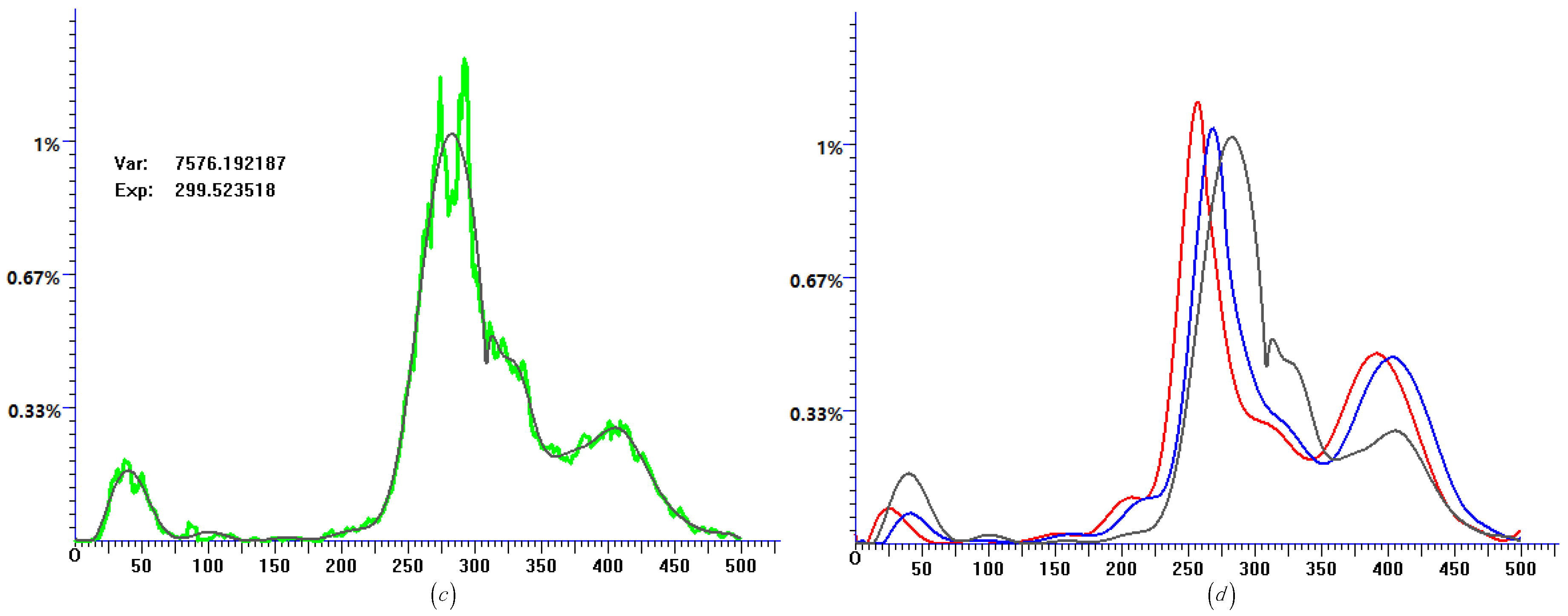
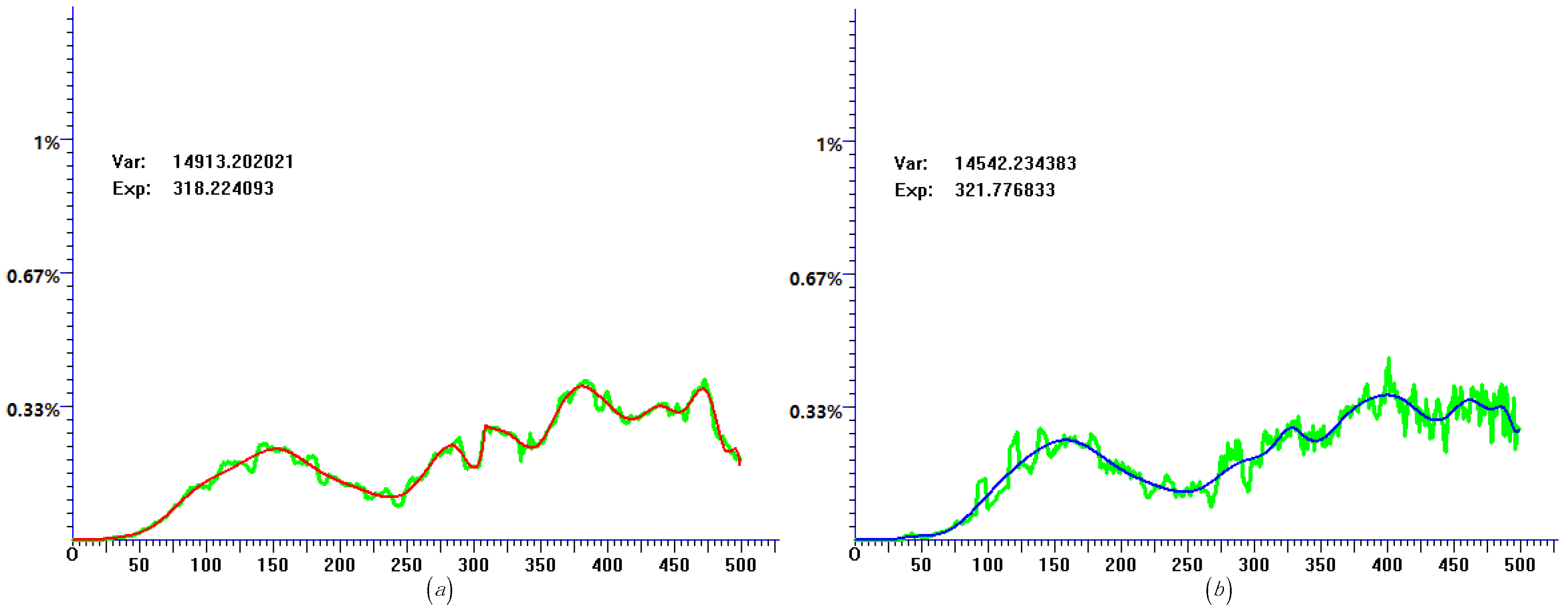
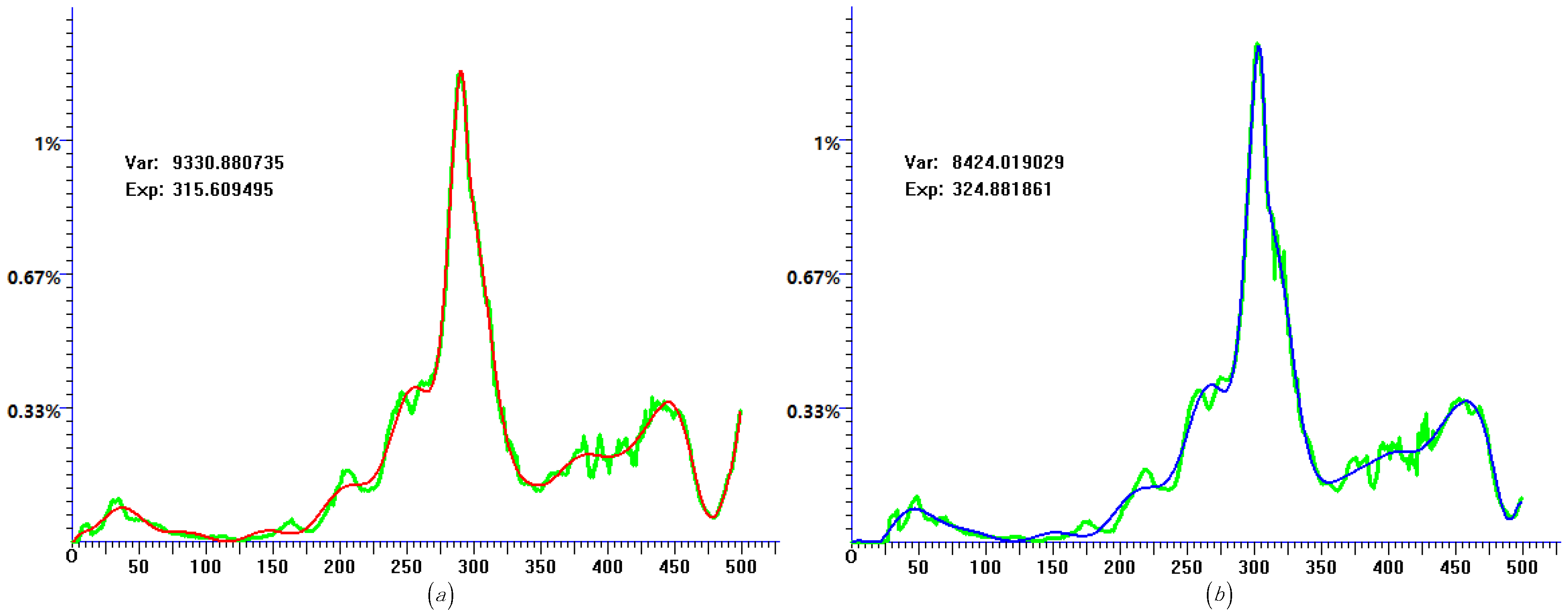
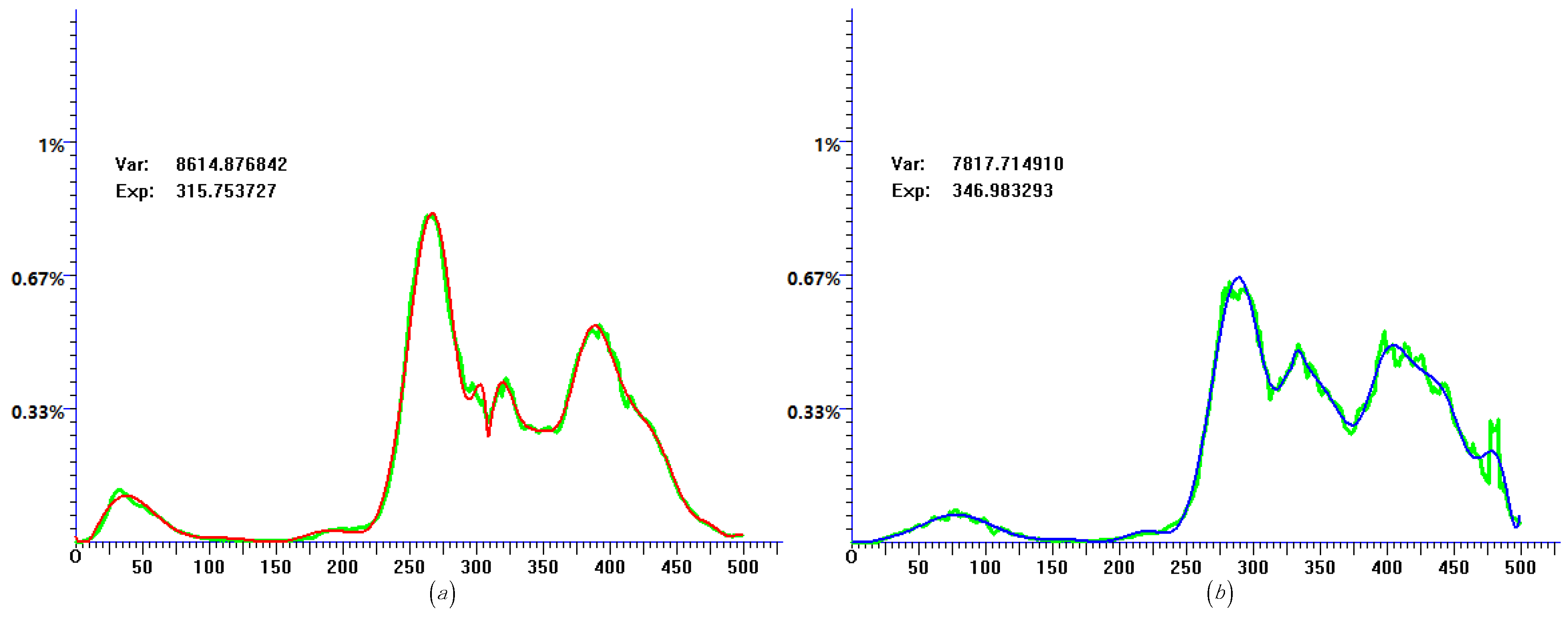
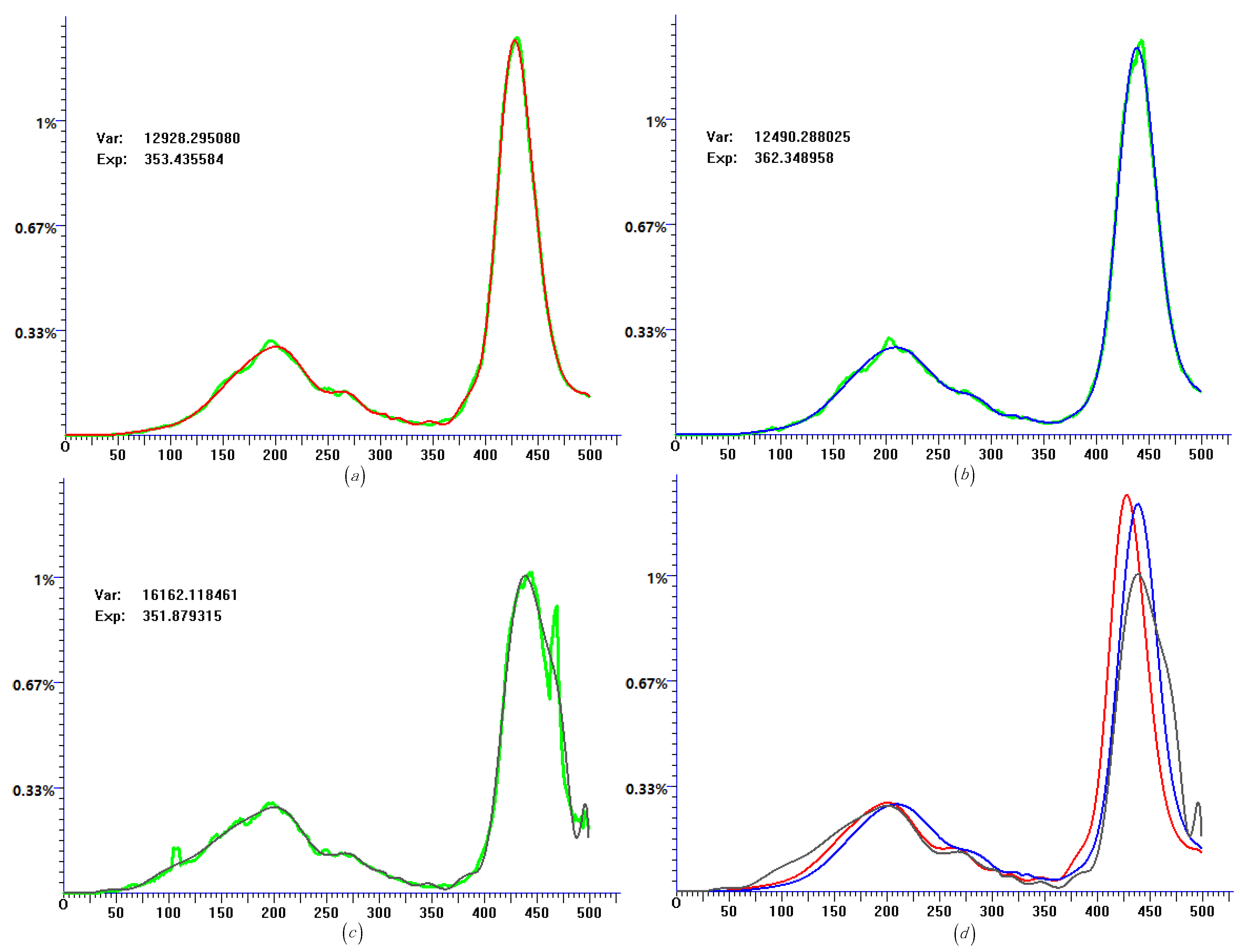
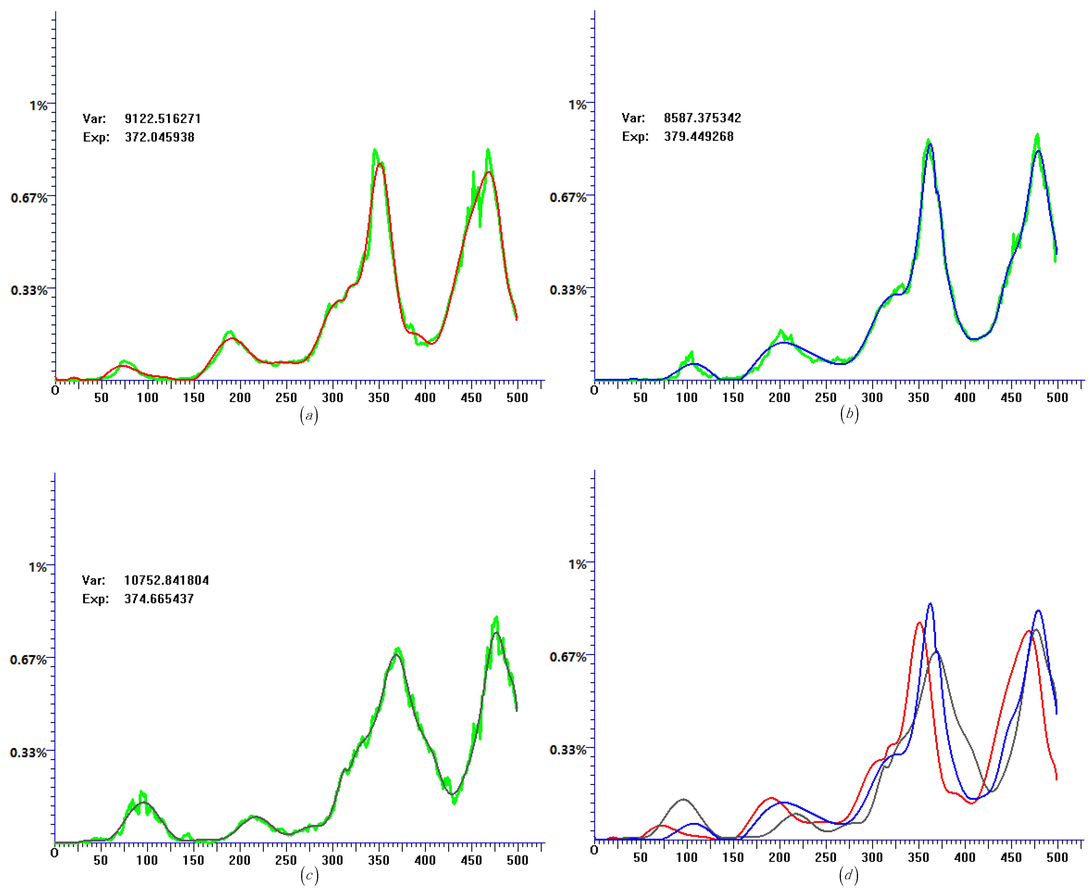
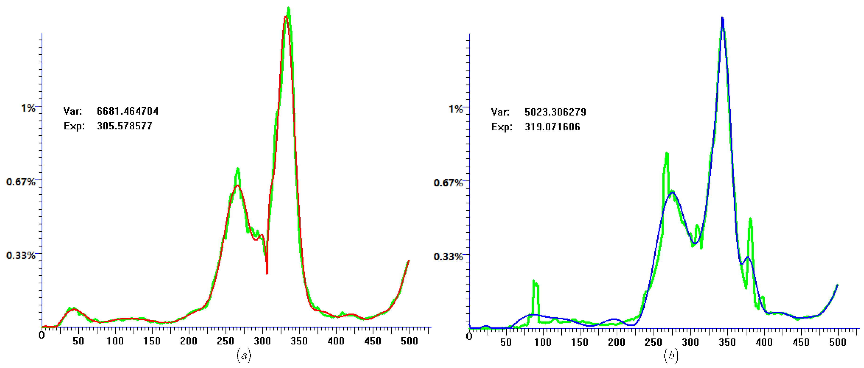
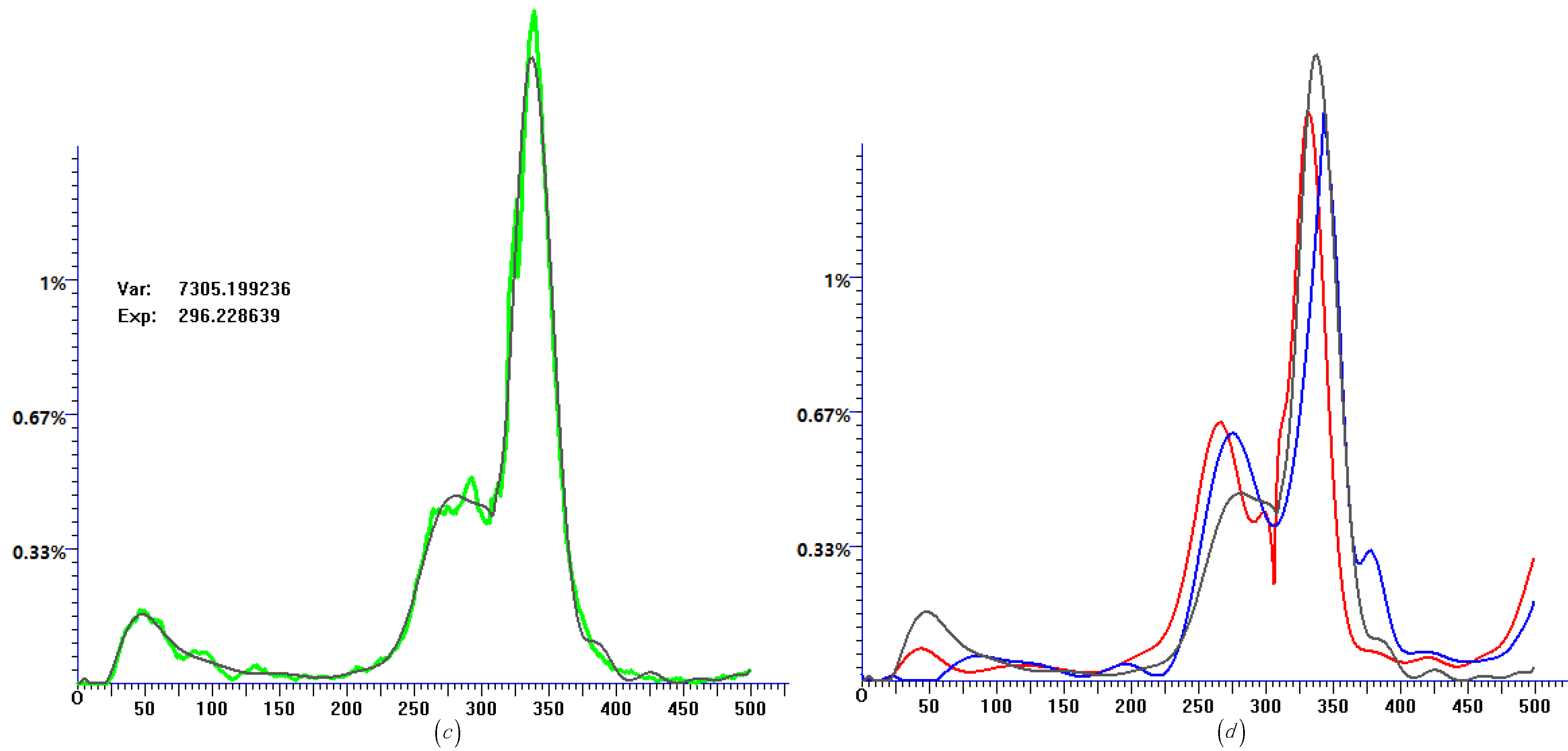
In this paper, we investigated eighteen countries’ COVID-19 data with the data interval of 500 days, and the quasi-distribution fitting results are shown in the following figures. In those figures, the green-colored signal denotes the 7-day moving average of the original data (called histogram data), including daily confirmed cases, daily recovery cases, and daily fatality cases. With the algorithm just presented, we obtain the corresponding quasi-distribution fitting results of those data, and put them together to find the inner trend of the pandemic. Figure 1 shows the experimental results of Austria. In Figure 1a, the red curve is the quasi-distribution fitting of the histogram data of daily confirmed cases; based on the previous definition, it could be regarded as the probability density function of daily confirmed cases if it was assumed to be a random variable. We can see from Figure 1a that the quasi-distribution curve fit the histogram data of daily conformed cases perfectly. Similarly, in Figure 1b, the blue curve is the quasi-distribution fitting of the histogram data of daily recovery cases, while in Figure 1c, the black curve is the quasi-distribution simulation of the histogram data of daily fatality cases. In Figure 1d, we put three fitting curves in the same coordinate: apparently, they all have three peaks, but at the first peak, the fatality curve is higher than the other two, while at the second peak there is no obvious difference, and at the third peak the fatality curve is quite a bit lower than the other two. This could mean that, as time goes on, even in the situation of the virus mutation, the case fatality rate of COVID-19 is continuing to decline, or it could be that this situation is only occurring in Austria, and the data of more countries need to be analyzed.

In the following figures, for every fitting scenario, the horizontal axis of the coordinate frame denotes the number of days, and the longitudinal axis denotes the percentage of the corresponding day’s data compared to the total data (sum of the whole 500 days of data), which is $f_k^{D}k=1,2,\cdots 500$ as mentioned previously in this paper.

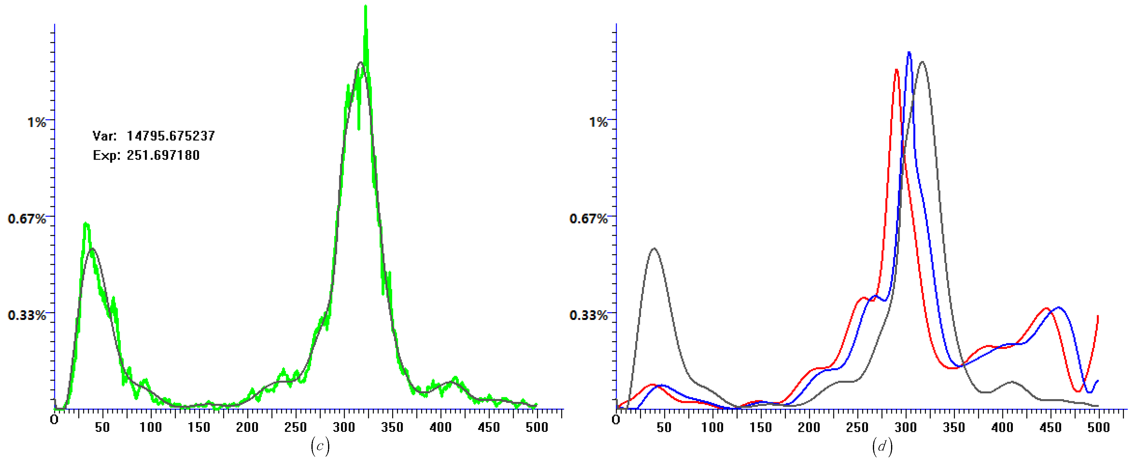
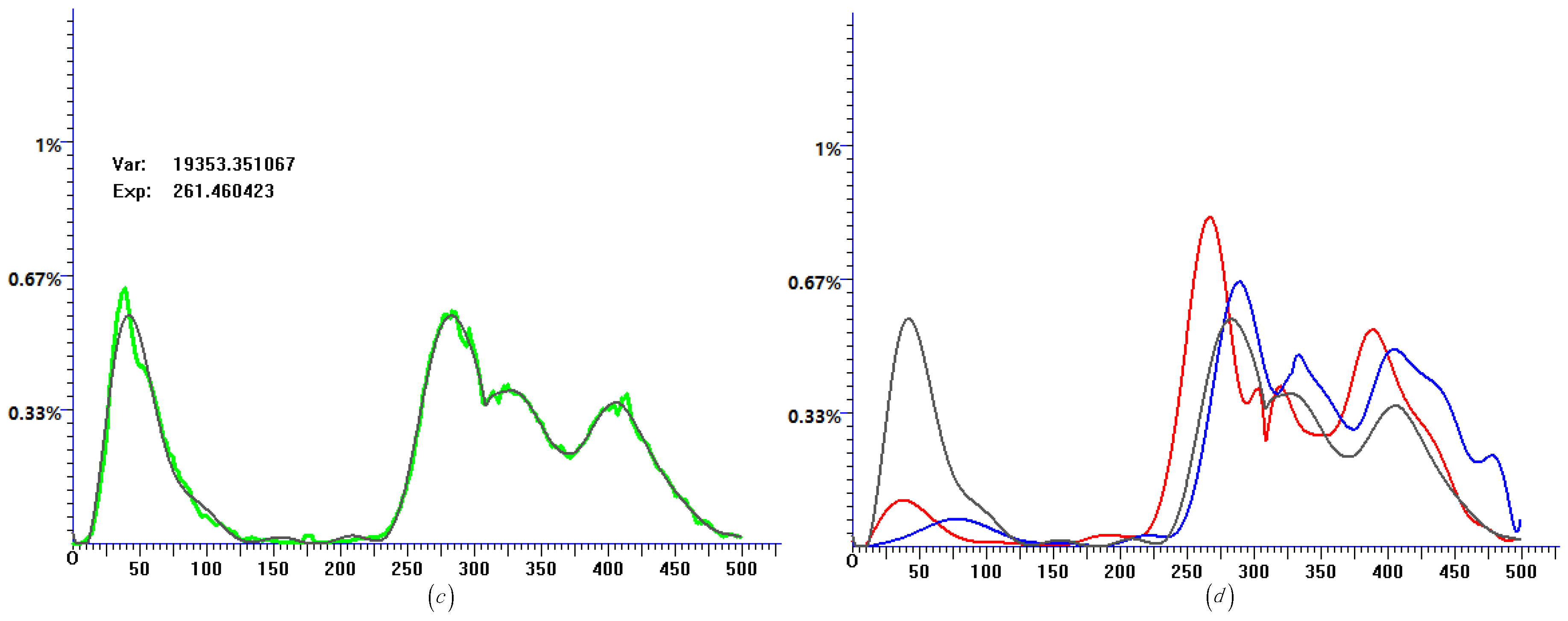
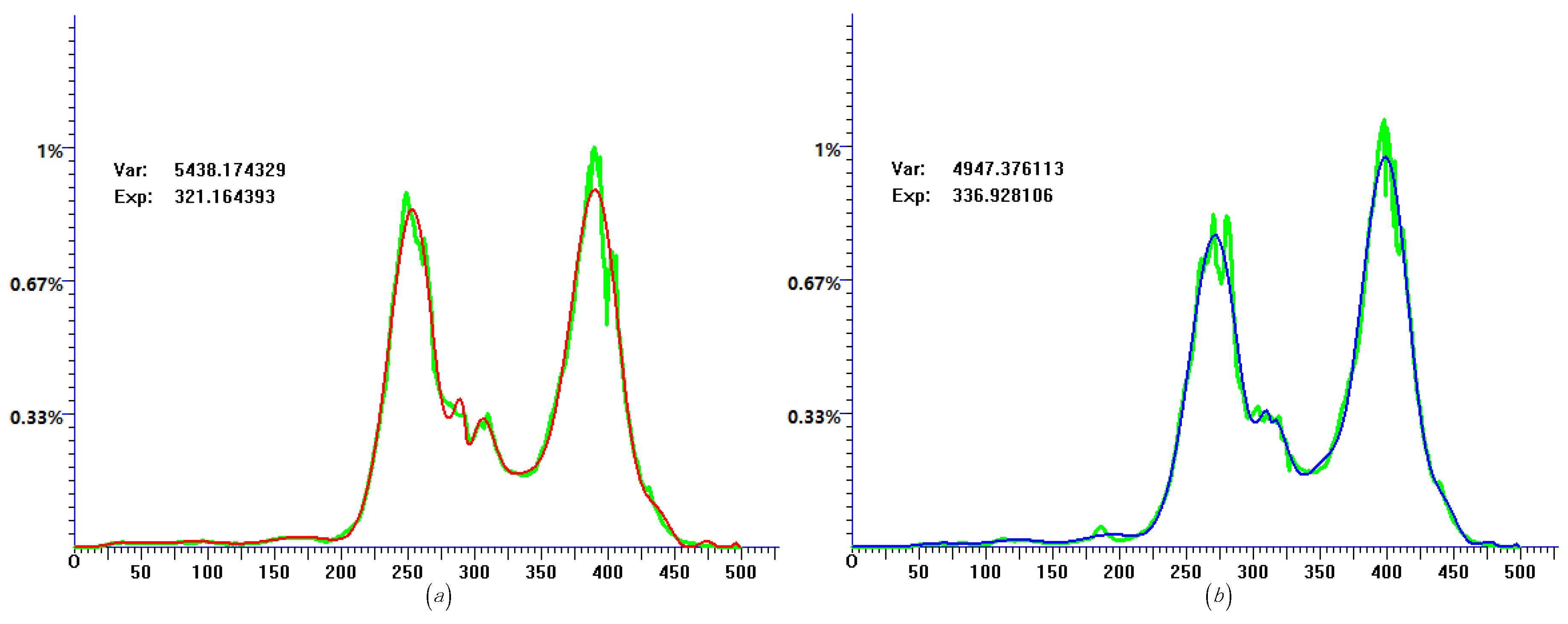
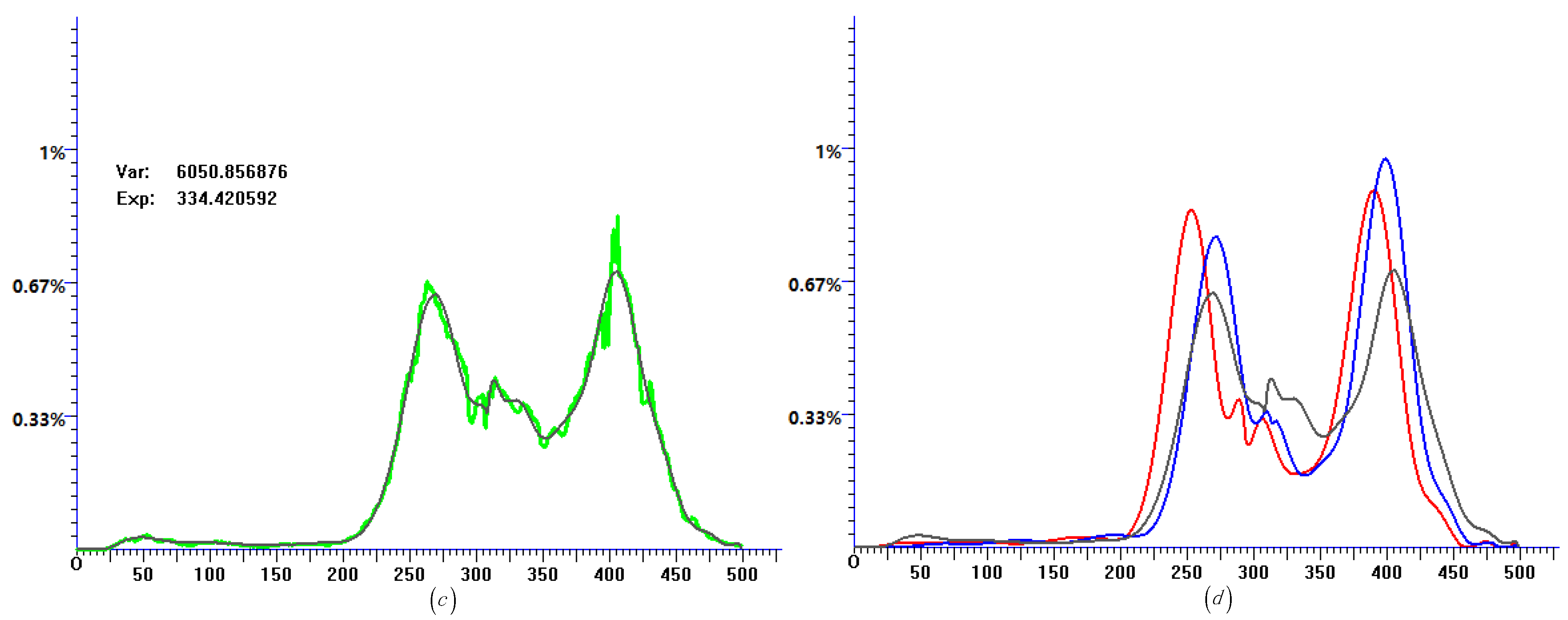
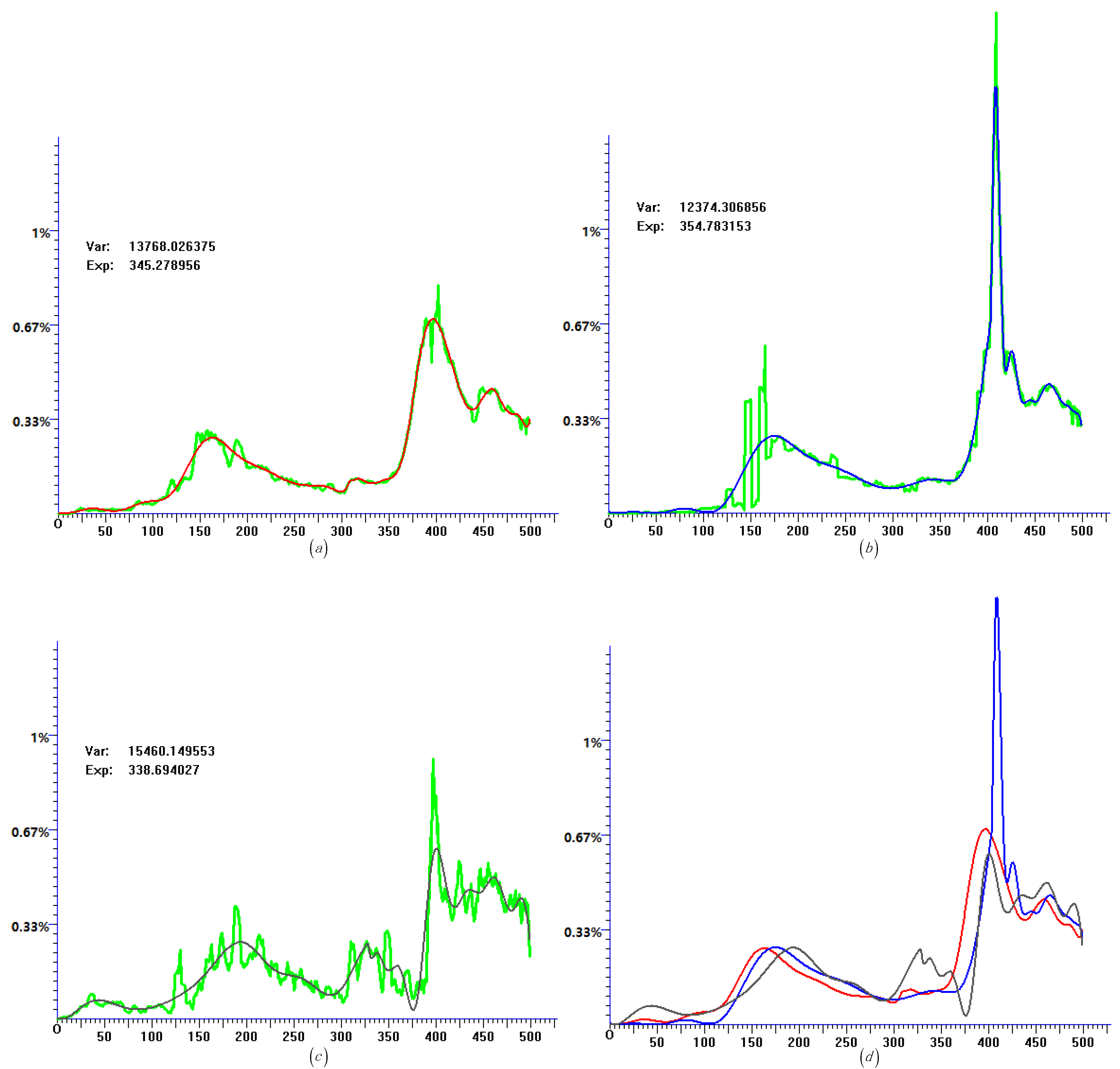
In Figure 2, we performed the same procedures on the data of Brazil, but the results were not similar to those of Austria, especially in Figure 2d, where the fatality peak around day 400 seems quite a bit higher than the previous peak around day 100, though the trend of quasi-distribution fitting curves of daily confirmed cases and daily recovery cases were still quite similar, so more countries’ data need to be included.

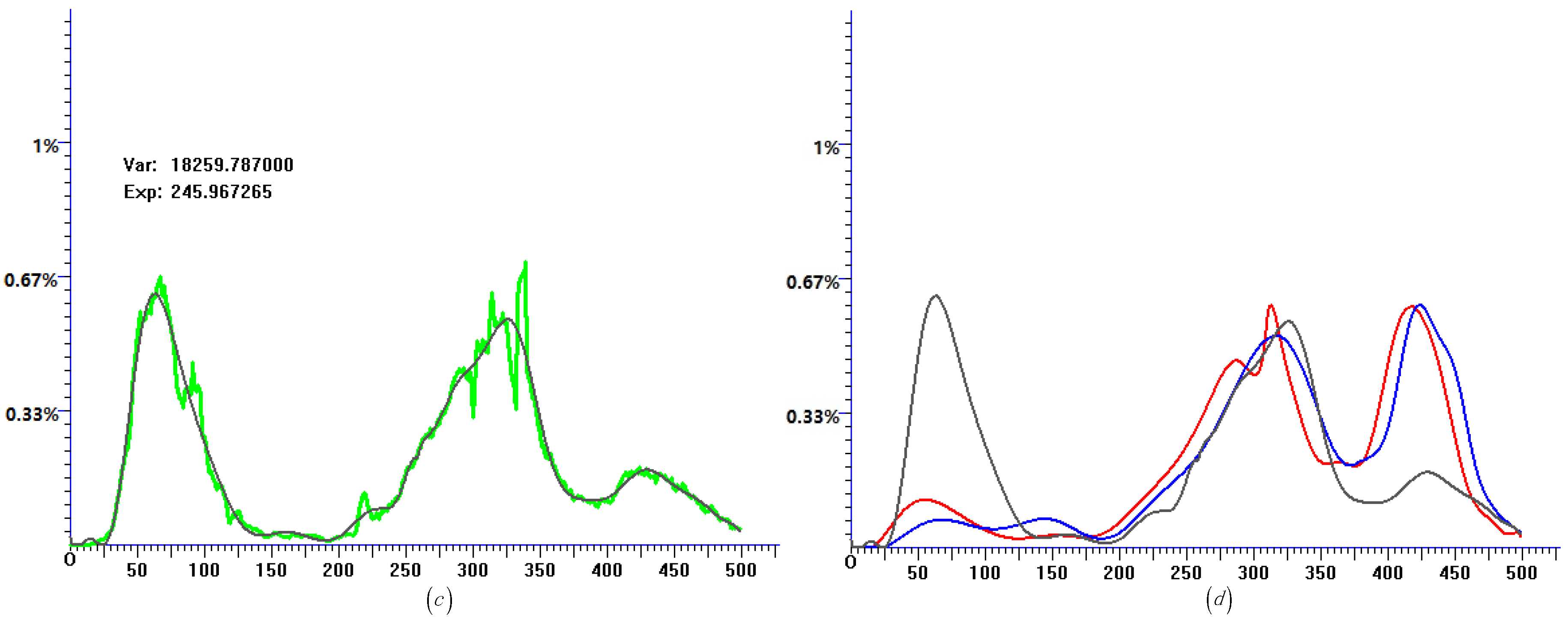
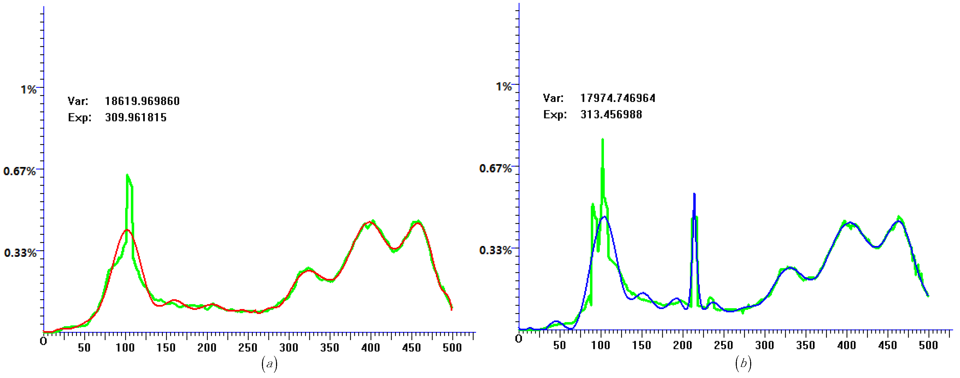
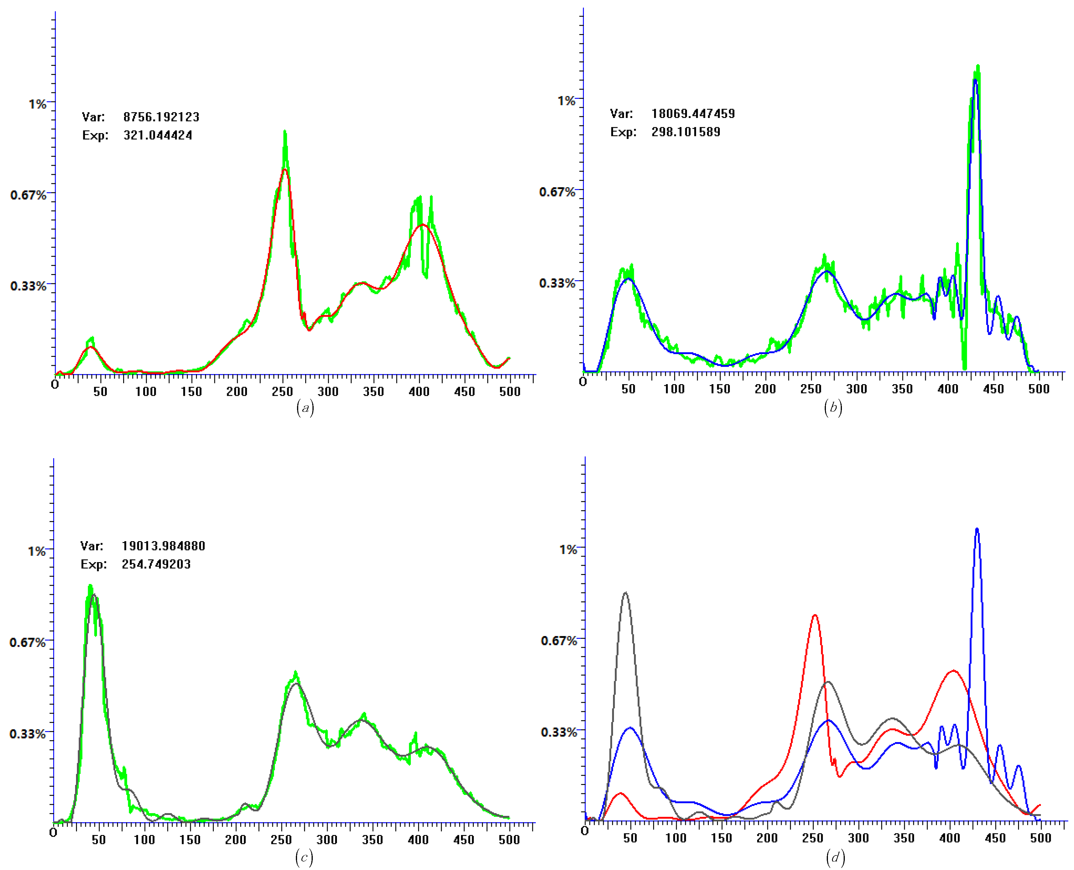
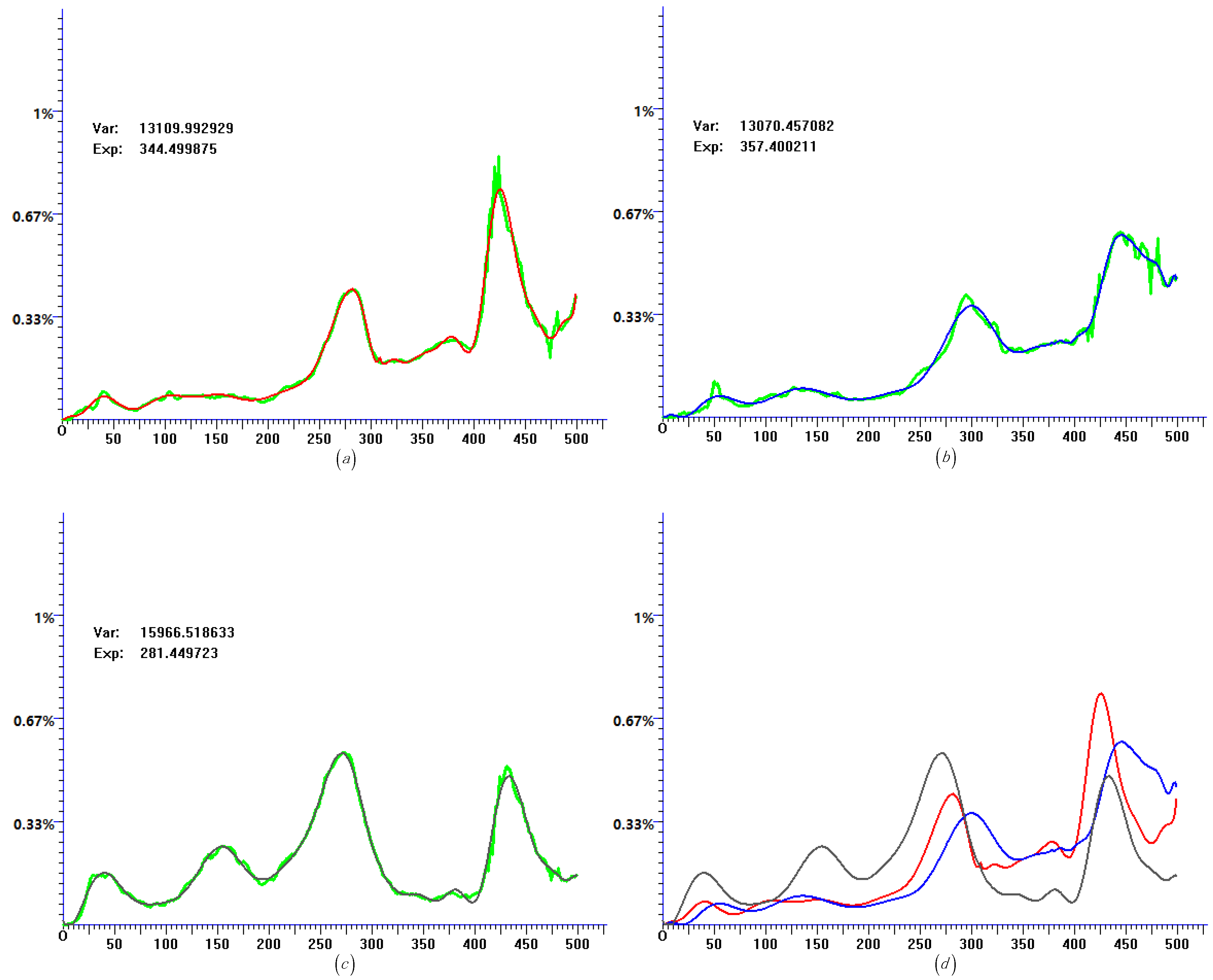
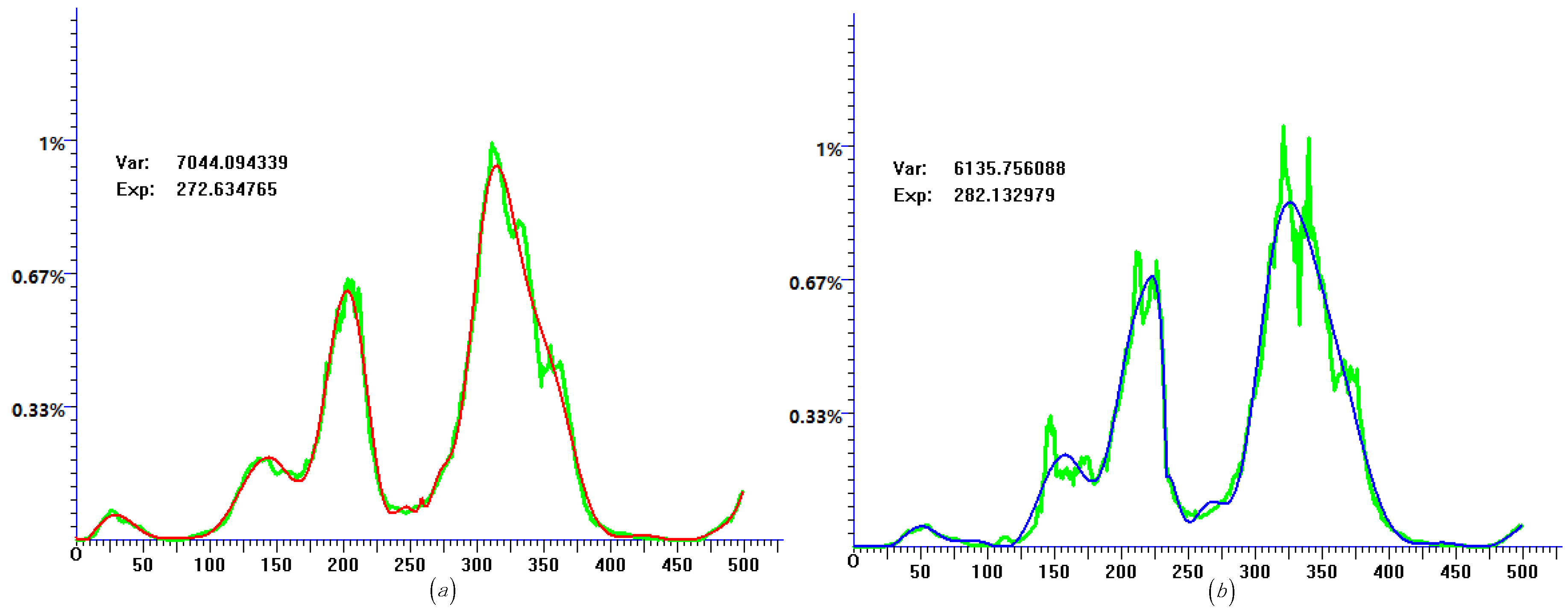
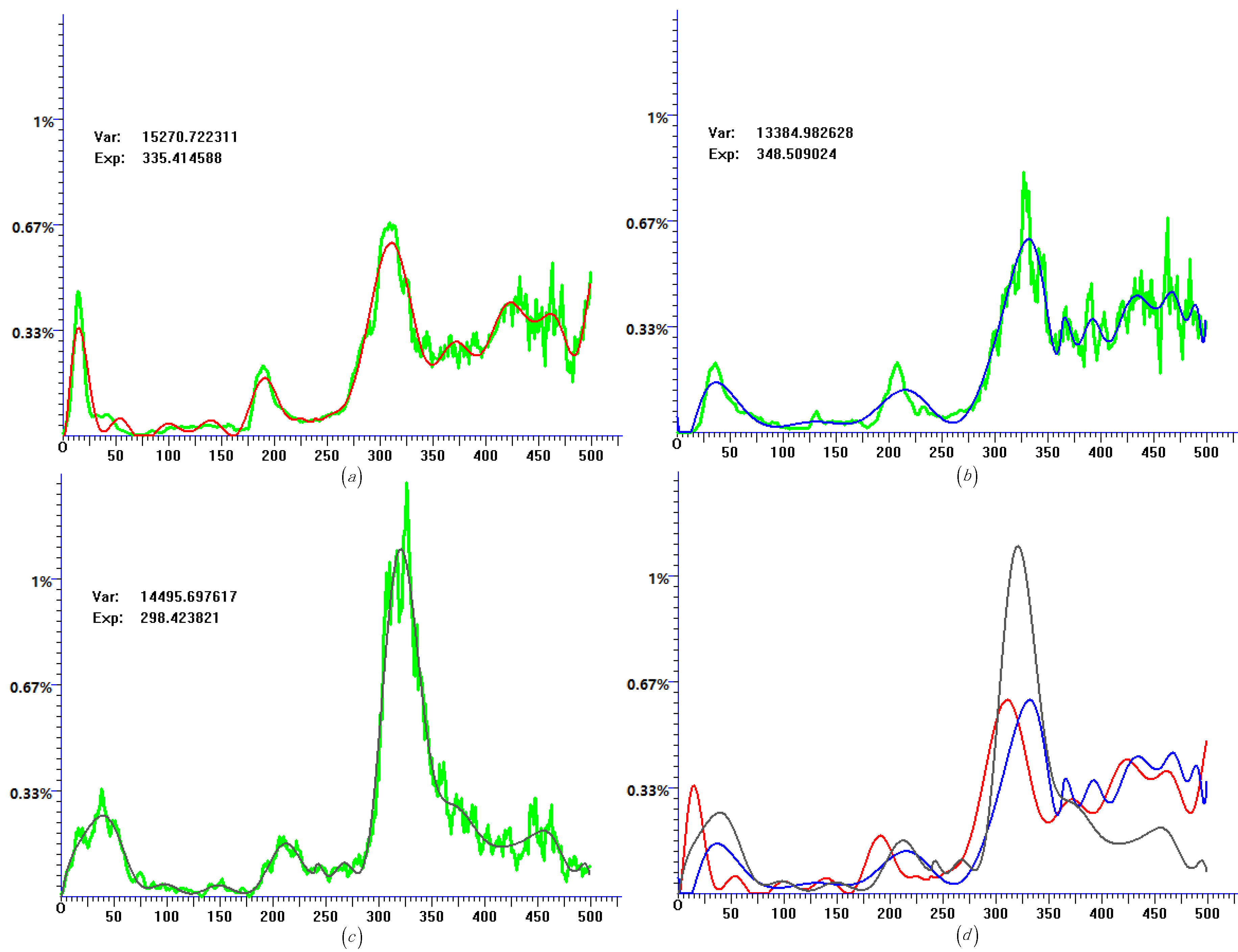
Figure 3 shows the experimental results of Canada, which shows the same results as Austria: in Figure 3d the third peak of the fatality curve is much lower than that of the daily confirmed cases and daily recovery cases, and in Figure 3b, around day 140 there is a boom in the daily recovery cases. Apparently, this is not because of a sudden increase in the medical system, but is rather due to the release of accumulated data; thus, we did not use the histogram data (7-day moving average data) to discover the inner trend of the pandemic, but instead used the corresponding quasi-distribution fitting curves.

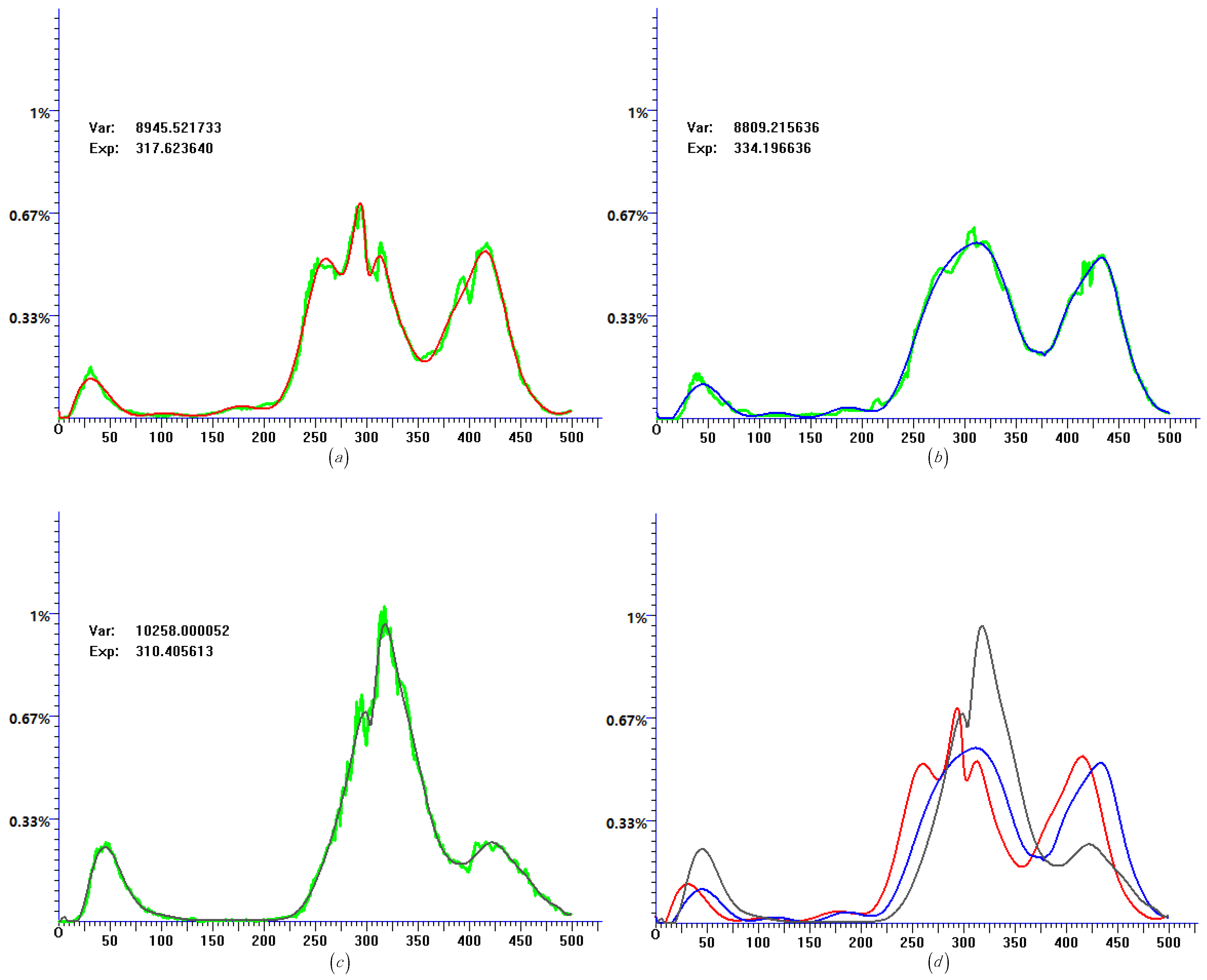
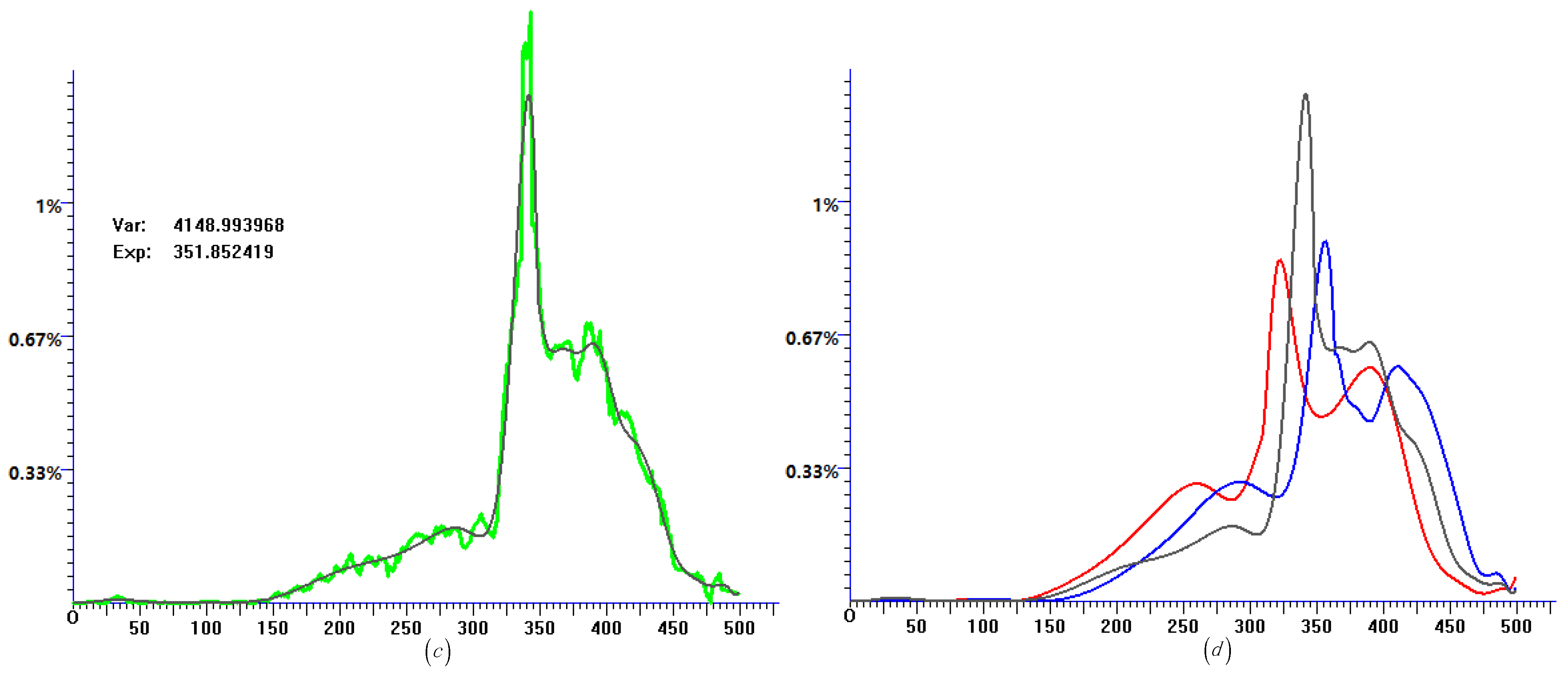
Figure 4 shows the situation in Chile; demonstrating the same results as those in Austria and Canada, the peak of the fatality curve in the later time is obviously lower than the peaks of the daily confirmed cases and daily recovery cases, showing the trend of the case fatality rate declining. Based on the value of “Var” (denoting the variance of the quasi-distribution fitting curve) in Figure 4a–c, the pandemic mode of Chile is quite similar to that of Brazil rather than that of Austria and Canada, perhaps because they are both located in South America and their geographical locations share the same climatic environment, affecting the spread of the epidemic.

Figure 5, Figure 6, Figure 7, Figure 8, Figure 9 and Figure 10 show the fitting results of epidemic data in Denmark, France, Germany, Italy, Iran, and the US, respectively, and they are almost the same as those in Austria and Canada, which demonstrates the fact that the third peak of the quasi-distribution fitting curve made by daily fatality cases obviously declined. Accordingly, it shows the fact that even with the spread of the epidemic, the fatality rate has clearly decreased.

Figure 11 shows the fitting results of India, from Figure 11a–c. For the daily confirmed cases, daily recovery cases, or daily fatality cases, the histogram data and their corresponding quasi-distribution fitting curves both only have two peaks, which does not mean that COVID-19 rarely spread during the first 50~70 days, but rather is due to the data around day 200 and day 430 (about the two peak points of the abscissa) are too large to make the early data obvious. In Figure 11d, we see that the second peak of the quasi-distribution fitting curve of daily fatalities is lower than that of the daily confirmed cases, showing the declining fatality rate of the pandemic. The same is true in Poland, as shown in Figure 12.

Figure 13 shows the fitting results of Israel, based on Figure 13d; even though the last peak of the quasi-distribution fitting curve of daily fatalities is lower than that of the daily confirmed cases (though not very obviously), so is the peak before the last one; therefore, we can draw the conclusion that, as time has gone on, the mortality rate has not increased in Israel. The epidemic situation in Japan and the Philippines is similar, as shown in Figure 14 and Figure 15, respectively.

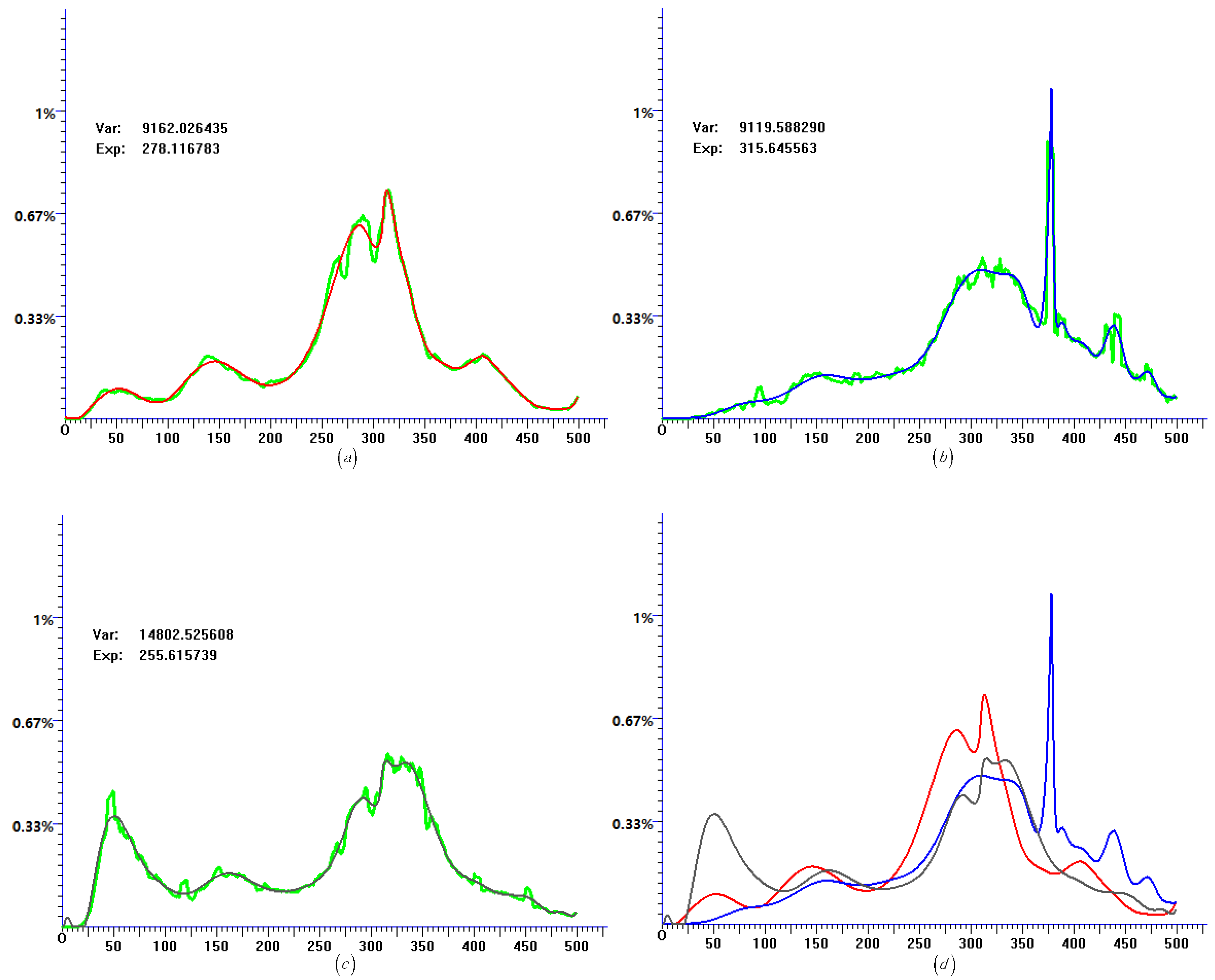
Figure 16 shows the fitting results of Korea; based on Figure 16d, the penultimate peak of the quasi-distribution fitting curve of daily fatalities is much higher than the other two fitting curves, but at the last peak, the quasi-distribution fitting curve of daily fatalities is obviously lower, which means the case fatality rate is declining at last. The epidemic situation in Lebanon and Portugal is similar, as shown in Figure 17 and Figure 18, respectively.

4. Conclusions

In this paper, we developed a new method, called the QDF method, to evaluate the spread of the epidemic caused by COVID-19 based on piecewise quasi-uniform B-spline curves. By fitting the distribution histogram data made from the daily confirmed cases, daily recovery cases, and daily fatality cases of eighteen countries, we came to the conclusion that with the spread of the epidemic, even in the situation of the virus mutation, the case fatality rate of the COVID-19 continues to decline. From the fitting results, the shape of the fitting curves of the daily recovery cases are very similar to the fitting curves of the daily confirmed cases, as shown in Figure 1a,b, Figure 2a,b, Figure 3a,b, Figure 5a,b, Figure 7a,b, Figure 8a,b, Figure 9a,b, Figure 11a,b, Figure 12a,b, Figure 13a,b, Figure 14a,b, Figure 16a,b, Figure 17a,b and Figure 18a,b; the corresponding fitting curves of daily recovery cases have delayed for certain days compared with their daily confirmed cases’ fitting curves, which means the treatment of the epidemic caused by COVID-19 has stabilized, and in the near future, the world will reopen.

References

- Zhu, N.; Zhang, D.; Wang, W.; Li, X.; Yang, B.; Song, J.; Zhao, X.; Huang, B.; Shi, W.; Lu, R.; et al. A novel coronavirus from patients with pneumonia in China, 2019. N. Engl. J. Med. 2020, 382, 727–733. [Google Scholar] [CrossRef] [PubMed]
- Zhou, P.; Yang, X.L.; Wang, X.G.; Hu, B.; Zhang, L.; Zhang, W.; Si, H.-L.; Zhu, Y.; Li, B.; Huang, C.-L.; et al. A pneumonia outbreak associated with a new coronavirus of probable bat origin. Nature 2020, 579, 270–273. [Google Scholar] [CrossRef] [PubMed] [Green Version]
- Krammer, F. SARS-CoV-2 vaccines in development. Nature 2020, 586, 516–527. [Google Scholar] [CrossRef] [PubMed]
- Rockx, B.; Kuiken, T.; Herfst, S.; Bestebroer, T.; Lamers, M.M.; Munnink, B.B.O.; De Meulder, D.; Van Amerongen, G.; Van Den Brand, J.; Okba, N.M.A.; et al. Comparative patheogenesis of COVID-19, MERS, and SARS in a nonhuman primate model. Science 2020, 368, 1012–1015. [Google Scholar] [CrossRef] [PubMed] [Green Version]
- Salahudeen, A.; Choi, S.S.; Rustagi, A.; Zhu, J.; van Unen, V.; Sean, M.; Flynn, R.A.; Margalef-Catala, M.; Santos, A.J.M.; Ju, J.; et al. Progenitor identification and SARS-CoV-2 infection in human distal lung organoids. Nature 2020, 588, 670–675. [Google Scholar] [CrossRef] [PubMed]
- Wolfer, R.; Corman, V.M.; Guggemos, W.; Seilmaier, M.; Zange, S.; Müller, M.A.; Niemeyer, D.; Janes, T.C.; Vollmar, P.; Rothe, C.; et al. Virological assessment of hospitalized patients with COVID-2019. Nature 2020, 581, 465–469. [Google Scholar] [CrossRef] [PubMed] [Green Version]
- Williamson, E.; Walker, A.J.; Bhaskaran, K.; Bacon, S.; Bates, C.; Morton, C.E.; Curtis, H.J.; Mehrkar, A.; Evans, D.; Inglesby, P.; et al. Factors associated with COVID-19-related death using OpenSAFELY. Nature 2020, 584, 430–436. [Google Scholar] [CrossRef] [PubMed]
- Gianicolo, E.; Russo, A.; Büchler, B.; Taylor, K.; Stang, A.; Blettner, M. Gender specific excess mortality in Italy during the COVID-19 pandemic accounting for age. Eur. J. Epidemiol. 2021, 52, 441–452. [Google Scholar] [CrossRef] [PubMed]
- Maness, S.; Merrell, L.; Thompson, E.L.; Griner, S.B.; Kline, N.; Wheldon, C. Social determinants of health and health disparites: COVID-19 exposures and mortality among African American people in the United States. Public Health Rep. 2021, 136, 18–22. [Google Scholar] [CrossRef] [PubMed]
- Lavezzo, E.; Franchin, E.; Ciavarella, C.; Cuomo-Dannenburg, G.; Barzon, L.; Del Vecchio, C.; Rossi, L.; Manganelli, R.; Loregian, A.; Navarin, N.; et al. Suppression of a SARS-CoV-2 outbreak in the Italian municipality of Vo’. Nature 2020, 584, 425–429. [Google Scholar] [CrossRef] [PubMed]
- Chang, S.; Pierson, E.; Koh, P.W.; Gerardin, J.; Redbird, B.; Grusky, D.; Leskovec, J. Mobility nextwork models of COVID-19 explain inequities and inform reopening. Nature 2021, 589, 82–87. [Google Scholar] [CrossRef] [PubMed]
- Hao, X.; Cheng, S.; Wu, D.; Wu, T.; Lin, X.; Wang, C. Reconstruction of the full transmission dynamics of COVID-19 in Wuhan. Nature 2020, 584, 420–424. [Google Scholar] [CrossRef] [PubMed]
- Hsiang, S.; Allen, D.; Annan-Phan, S.; Bell, K.; Bolliger, I.; Chong, T.; Druckenmiller, H.; Huang, L.Y.; Hultgren, A.; Krasovich, E.; et al. The effect of large-scale anti-contagion policies on the COVID-19 pandemic. Nature 2020, 584, 262–267. [Google Scholar] [CrossRef] [PubMed]
- Flaxman, S.; Van Weenen, E.; Lison, A.; Cenedese, A.; Seeliger, A.; Kratzwald, B.; Whittaker, C.; Zhu, H.; Berah, T.; Eatin, J.W.; et al. Estimating the effects of non-pharmaceutical interventions on COVID-19 in Europe. Nature 2020, 584, 257–261. [Google Scholar] [CrossRef] [PubMed]
- Plumper, T.; Neumayer, E. The pandemic predominantly hits poor neighbourhoods? SARS-CoV-2 infections and COVID-19 fatalites in German districts. Eur. J. Public Health 2020, 30, 1176–1180. [Google Scholar]
- Pisot, S.; Milovanović, I.; Šimunič, B.; Gentile, A.; Bosnar, K.; Prot, F.; Bianco, A.; Coco, G.L.; Bartoluci, S.; Katović, D.; et al. Maintaining everyday life praxis in the time of COVID-19 pandemic measures (ELP-COVID-19 survey). Eur. J. Public Health 2020, 30, 1181–1186. [Google Scholar] [CrossRef] [PubMed]
- O’Driscoll, M.; Dos Santos, G.R.; Wang, L.; Cummings, D.A.; Azman, A.S.; Paireau, J.; Fontanet, A.; Cauchemez, S.; Salje, H. Age-specific mortality and immunity patterns of SARS-CoV-2. Nature 2021, 590, 262–267. [Google Scholar] [CrossRef] [PubMed]
- Wang, Y.D.; Hu, B.F.; Xi, P.; Xue, W. A note on variable upper limit integral of Bezier curve. Adv. Sci. Lett. 2011, 4, 2986–2990. [Google Scholar] [CrossRef]
Figure 1.
Histogram data and quasi-distribution fitting of Austria. (a) Histogram data of daily confirmed cases and the corresponding quasi-distribution fitting. (b) Histogram data of daily recovery cases and the corresponding quasi-distribution fitting. (c) Histogram data of daily fatality cases and the corresponding quasi-distribution fitting. (d) Quasi-distribution fitting results of daily confirmed cases (red), daily recovery cases (blue), and daily fatality cases (black) show in the same coordinate.
Figure 2.
Histogram data and quasi-distribution fitting of Brazil. (a) Histogram data of daily confirmed cases and the corresponding quasi-distribution fitting. (b) Histogram data of daily recovery cases and the corresponding quasi-distribution fitting. (c) Histogram data of daily fatality cases and the corresponding quasi-distribution fitting. (d) Quasi-distribution fitting results of daily confirmed cases (red), daily recovery cases (blue), and daily fatality cases (black) show in the same coordinate.
Figure 3.
Histogram data and quasi-distribution fitting of Canada. (a) Histogram data of daily confirmed cases and the corresponding quasi-distribution fitting. (b) Histogram data of daily recovery cases and the corresponding quasi-distribution fitting. (c) Histogram data of daily fatality cases and the corresponding quasi-distribution fitting. (d) Quasi-distribution fitting results of daily confirmed cases (red), daily recovery cases (blue), and daily fatality cases (black) show in the same coordinate.
Figure 4.
Histogram data and quasi-distribution fitting of Chile. (a) Histogram data of daily confirmed cases and the corresponding quasi-distribution fitting. (b) Histogram data of daily recovery cases and the corresponding quasi-distribution fitting. (c) Histogram data of daily fatality cases and the corresponding quasi-distribution fitting. (d) Quasi-distribution fitting results of daily confirmed cases (red), daily recovery cases (blue), and daily fatality cases (black) show in the same coordinate.
Figure 5.
Histogram data and quasi-distribution fitting of Denmark. (a) Histogram data of daily confirmed cases and the corresponding quasi-distribution fitting. (b) Histogram data of daily recovery cases and the corresponding quasi-distribution fitting. (c) Histogram data of daily fatality cases and the corresponding quasi-distribution fitting. (d) Quasi-distribution fitting results of daily confirmed cases (red), daily recovery cases (blue), and daily fatality cases (black) show in the same coordinate.
Figure 6.
Histogram data and quasi-distribution fitting of France. (a) Histogram data of daily confirmed cases and the corresponding quasi-distribution fitting. (b) Histogram data of daily recovery cases and the corresponding quasi-distribution fitting. (c) Histogram data of daily fatality cases and the corresponding quasi-distribution fitting. (d) Quasi-distribution fitting results of daily confirmed cases (red), daily recovery cases (blue), and daily fatality cases (black) show in the same coordinate.
Figure 7.
Histogram data and quasi-distribution fitting of Germany. (a) Histogram data of daily confirmed cases and the corresponding quasi-distribution fitting. (b) Histogram data of daily recovery cases and the corresponding quasi-distribution fitting. (c) Histogram data of daily fatality cases and the corresponding quasi-distribution fitting. (d) Quasi-distribution fitting results of daily confirmed cases (red), daily recovery cases (blue), and daily fatality cases (black) show in the same coordinate.
Figure 8.
Histogram data and quasi-distribution fitting of Italy. (a) Histogram data of daily confirmed cases and the corresponding quasi-distribution fitting. (b) Histogram data of daily recovery cases and the corresponding quasi-distribution fitting. (c) Histogram data of daily fatality cases and the corresponding quasi-distribution fitting. (d) Quasi-distribution fitting results of daily confirmed cases (red), daily recovery cases (blue), and daily fatality cases (black) show in the same coordinate.
Figure 9.
Histogram data and quasi-distribution fitting of Iran. (a) Histogram data of daily confirmed cases and the corresponding quasi-distribution fitting. (b) Histogram data of daily recovery cases and the corresponding quasi-distribution fitting. (c) Histogram data of daily fatality cases and the corresponding quasi-distribution fitting. (d) Quasi-distribution fitting results of daily confirmed cases (red), daily recovery cases (blue), and daily fatality cases (black) show in the same coordinate.
Figure 10.
Histogram data and quasi-distribution fitting of the US. (a) Histogram data of daily confirmed cases and the corresponding quasi-distribution fitting. (b) Histogram data of daily recovery cases and the corresponding quasi-distribution fitting. (c) Histogram data of daily fatality cases and the corresponding quasi-distribution fitting. (d) Quasi-distribution fitting results of daily confirmed cases (red), daily recovery cases (blue), and daily fatality cases (black) show in the same coordinate.
Figure 11.
Histogram data and quasi-distribution fitting of India. (a) Histogram data of daily confirmed cases and the corresponding quasi-distribution fitting. (b) Histogram data of daily recovery cases and the corresponding quasi-distribution fitting. (c) Histogram data of daily fatality cases and the corresponding quasi-distribution fitting. (d) Quasi-distribution fitting results of daily confirmed cases (red), daily recovery cases (blue), and daily fatality cases (black) show in the same coordinate.
Figure 12.
Histogram data and quasi-distribution fitting of Poland. (a) Histogram data of daily confirmed cases and the corresponding quasi-distribution fitting. (b) Histogram data of daily recovery cases and the corresponding quasi-distribution fitting. (c) Histogram data of daily fatality cases and the corresponding quasi-distribution fitting. (d) Quasi-distribution fitting results of daily confirmed cases (red), daily recovery cases (blue), and daily fatality cases (black) show in the same coordinate.
Figure 13.
Histogram data and quasi-distribution fitting of Israel. (a) Histogram data of daily confirmed cases and the corresponding quasi-distribution fitting. (b) Histogram data of daily recovery cases and the corresponding quasi-distribution fitting. (c) Histogram data of daily fatality cases and the corresponding quasi-distribution fitting. (d) Quasi-distribution fitting results of daily confirmed cases (red), daily recovery cases (blue), and daily fatality cases (black) show in the same coordinate.
Figure 14.
Histogram data and quasi-distribution fitting of Japan. (a) Histogram data of daily confirmed cases and the corresponding quasi-distribution fitting. (b) Histogram data of daily recovery cases and the corresponding quasi-distribution fitting. (c) Histogram data of daily fatality cases and the corresponding quasi-distribution fitting. (d) Quasi-distribution fitting results of daily confirmed cases (red), daily recovery cases (blue), and daily fatality cases (black) show in the same coordinate.
Figure 15.
Histogram data and quasi-distribution fitting of the Philippines. (a) Histogram data of daily confirmed cases and the corresponding quasi-distribution fitting. (b) Histogram data of daily recovery cases and the corresponding quasi-distribution fitting. (c) Histogram data of daily fatality cases and the corresponding quasi-distribution fitting. (d) Quasi-distribution fitting results of daily confirmed cases (red), daily recovery cases (blue), and daily fatality cases (black) show in the same coordinate.
Figure 16.
Histogram data and quasi-distribution fitting of Korea. (a) Histogram data of daily confirmed cases and the corresponding quasi-distribution fitting. (b) Histogram data of daily recovery cases and the corresponding quasi-distribution fitting. (c) Histogram data of daily fatality cases and the corresponding quasi-distribution fitting. (d) Quasi-distribution fitting results of daily confirmed cases (red), daily recovery cases (blue), and daily fatality cases (black) show in the same coordinate.
Figure 17.
Histogram data and quasi-distribution fitting of Lebanon. (a) Histogram data of daily confirmed cases and the corresponding quasi-distribution fitting. (b) Histogram data of daily recovery cases and the corresponding quasi-distribution fitting. (c) Histogram data of daily fatality cases and the corresponding quasi-distribution fitting. (d) Quasi-distribution fitting results of daily confirmed cases (red), daily recovery cases (blue), and daily fatality cases (black) show in the same coordinate.
Figure 18.
Histogram data and quasi-distribution fitting of Portugal. (a) Histogram data of daily confirmed cases and the corresponding quasi-distribution fitting. (b) Histogram data of daily recovery cases and the corresponding quasi-distribution fitting. (c) Histogram data of daily fatality cases and the corresponding quasi-distribution fitting. (d) Quasi-distribution fitting results of daily confirmed cases (red), daily recovery cases (blue), and daily fatality cases (black) show in the same coordinate.