
The COVID-19 Pandemic and Dynamics of Price Adjustment in the U.S. Beef Sector


Department of Agricultural Economics, University of Kentucky, Lexington, KY 40546, USA
*
Author to whom correspondence should be addressed.
Sustainability 2022, 14(8), 4391; https://doi.org/10.3390/su14084391
Submission received: 20 February 2022
/
Revised: 29 March 2022
/
Accepted: 5 April 2022
/
Published: 7 April 2022
(This article belongs to the Special Issue Economic and Social Consequences of the COVID-19 Pandemic)
Abstract
:This research investigates the impact of the COVID-19 pandemic on the dynamics of vertical price transmission in the U.S. beef industry using monthly farm, wholesale, and retail prices for the period 1970–2021. Contemporary time-series techniques and historical decomposition graphs were used to test for possible asymmetries and structural breaks in the price transmission across the beef supply chain. The results show that the impact of COVID-19 has been uneven across the beef marketing channel, with consumers and farmers sharing the burden of the shock. Historical decomposition graphs demonstrated that the COVID-19 pandemic caused consumers paying higher prices, but farmers receiving lower prices than their predicted values. Hence, both consumers and farmers in the U.S. beef supply chain were adversely affected by the COVID-19 pandemic. Furthermore, the results detected asymmetric price adjustments along the U.S. beef supply chain, both in speeds and magnitudes, with the wholesale prices being more flexible, adjusting quicker than farm and retail prices. The results indicated that the U.S. beef markets were resilient enough to absorb the shock and return to their pre-shock patterns in 4 to 6 months. These results have welfare and policy implications for the U.S. beef industry.
1. Introduction
SARS-CoV-2 which turned into coronavirus disease in 2019 (COVID-19), was first detected in December of 2019 in China. The global impact was realized in March 2020 after the World Health Organization announced it as a global pandemic. COVID-19 has caused devastating health, social, and economic problems across the world, in contrast with other members of coronaviruses family: severe acute respiratory syndrome-SARS and Middle East respiratory syndrome-MERS [1]. The first federal policy response in the U.S. was the declaration of a national emergency by President Trump on 19 March 2020. On 27 March 2020, the U.S. Senate passed a $2 trillion Coronavirus Aid Relief, and an Economic Security (CARES) Act to support hospitals, small businesses, and state and local governments.
United States is the largest producer and consumer of beef in the world with 20% of the global beef production [2]. Total beef supply in the U.S. was 27.6 billion pounds and the number of beef cows was 31.3 million in 2020 [3]. The main stages of beef-cattle production process in U.S. are cow-calf operations, stocker/backgrounding operations, feedlots, meat packers and processors, and retailers. The production process begins with the cow-calf farms where cows and calves are raised. The next stage of production occurs at stocker/backgrounding operations where calves are placed on grass or other type of roughage. Feedlots are the final chain in the cattle production and they feed cattle with different rations of grain, silage, and/or protein supplements and sell to beef packers and processors where beef and beef by-products are produced and sold to retailers [4]. The economic size of beef-cattle industry including direct and indirect economic contributions during on-farm and post-farm activities is estimated as $167 billion in 2016 [5]. Although U.S. has one of the largest cow herd and the largest beef production amounts in the world, it was net importer in beef trade with export amount of 3.0 million pounds and import amount of 3.3 million pounds in 2020 [3]. In addition to economic value, beef is also an indispensable nutrition in American dietary behaviors. It is a highly nutritious food as a source of protein, zinc, iron, and other minerals, B vitamins and choline. Consumers have different types of beef whose quality standards are regulated and monitored by USDA. Beef quality grading is vital in purchasing behaviors and it is based on tenderness, juiciness, and flavor. There are eight quality grades in U.S. grading system: U.S. Prime, U.S. Choice, U.S. Select, U.S. Standard, U.S. Commercial, U.S. Utility, U.S. Cutter, and U.S. Canner. U.S. Prime has the highest and U.S. Canner has the lowest quality.
During the COVID-19 pandemic, we have observed unexpected price movements in the U.S. beef market due to the disruptions in the beef marketing channel. The supply chain disruptions in the U.S. beef market were first experienced at the beef packing plants and processors due to the spread of COVID-19 among the workers, which caused temporarily shutdowns of some plants and capacity limitations at some facilities [6,7]. These shutdowns and capacity shortages at the wholesale level resulted in price hikes at the wholesale and retail levels, and oversupply, lower prices, and income losses at the farm level [8].
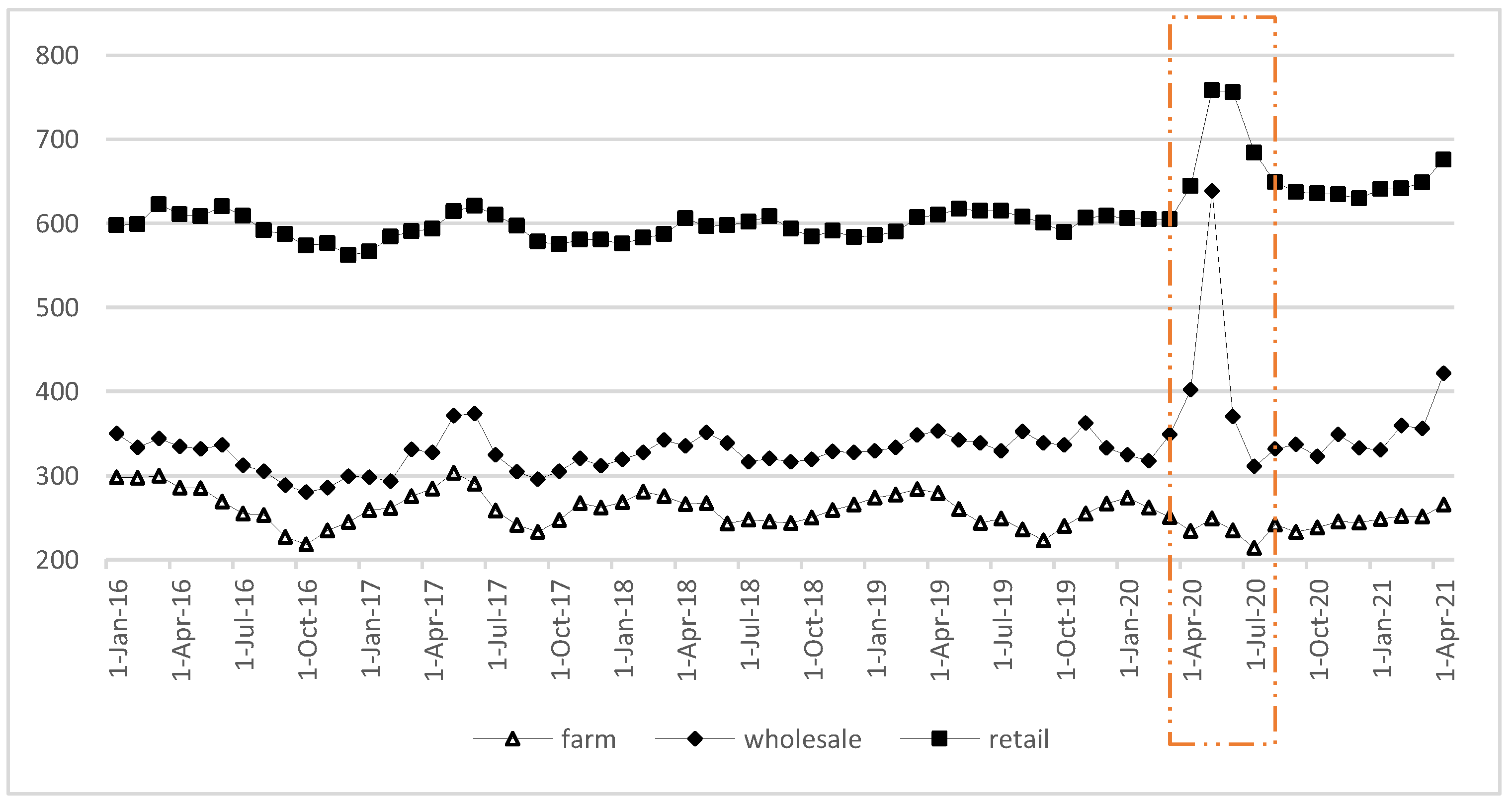
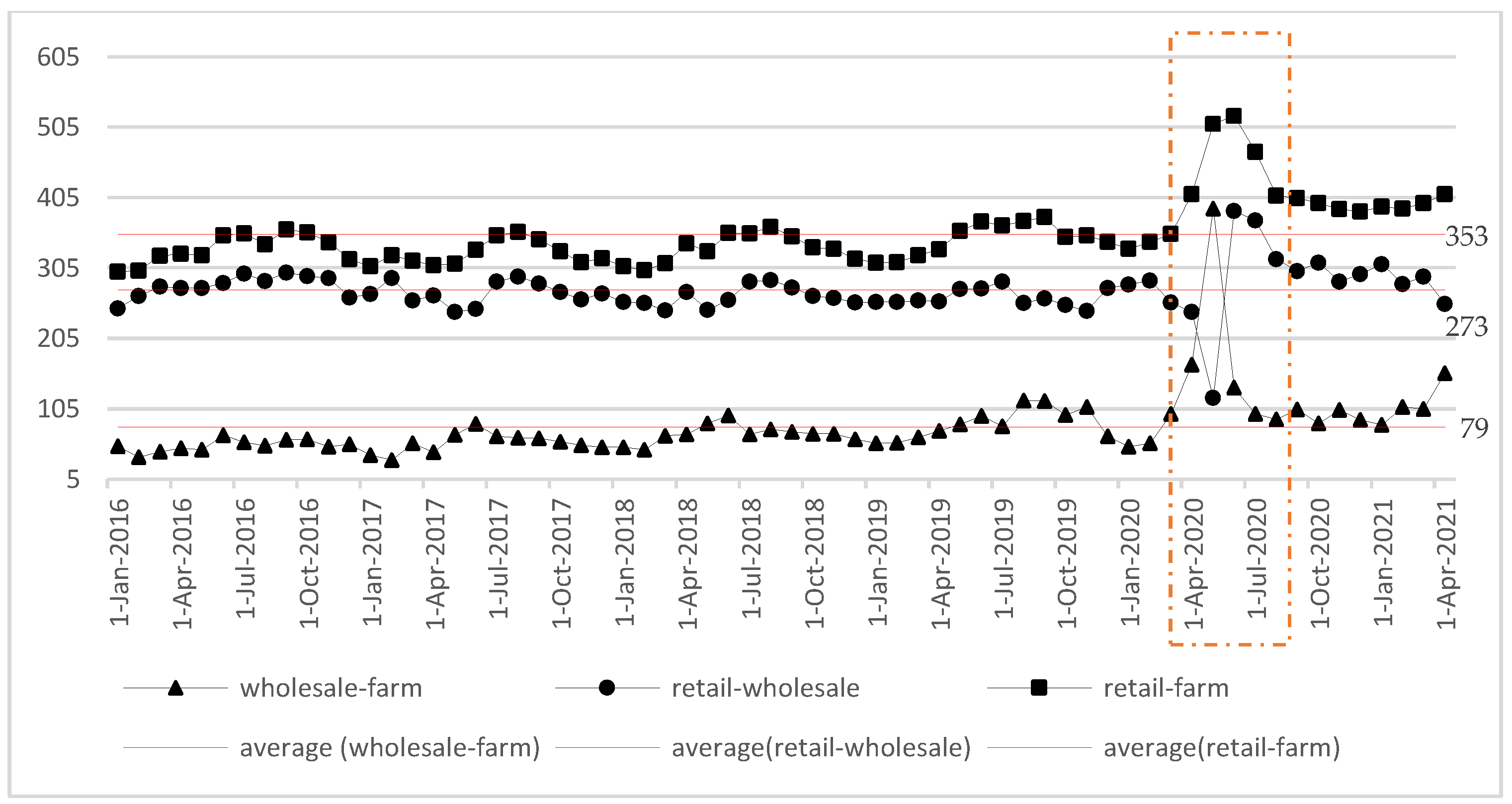
Figure 1 and Figure 2 depict the changes in the U.S. beef prices and price spreads. Price hikes were observed between March and May 2020 for wholesale prices and between March and June 2020 for retail prices (Figure 1, the colored line box). The increase is 58.9% in wholesale prices and 17.7% in retail prices in May 2020. Although price decreases at farm level started before pandemic, it worsened between March–July 2020. The impact on the price spreads are also worth mentioning. Wholesale-farm price spread started at 98 cents per dollar in May 2020, and jumps to 389 cents per dollar. Although it decreased to 97 cents per dollar after two months, it remained above the average value of the period January 2016–April 2021 (Figure 2, the colored line box). We observe the opposite movements in the retail-wholesale price spreads. Retail-farm and retail-wholesale price spreads stayed above their averages after the initial pandemic effect.
In this study, we investigate the type, magnitude and speed of price adjustments under the COVID-19 pandemic shock along the beef marketing channel with different econometric methods. In addition to changes in prices and price spreads, we utilize a vector error correction (VEC) model with structural breaks and historical decomposition graphs to investigate the impact of the COVID-19 pandemic shock on the short-run dynamics and speeds of price adjustment along the U.S. beef marketing channel to examine how the pandemic affected the adjustment patterns along the beef supply channel. In addition, we investigate the long-run relationships among the farm, wholesale and retail beef prices. The long-run convergence of the price series could point to market efficiency and integration of the beef marketing channel. Price adjustment along the farm, wholesale, and retail levels, and its impact on the economic agents across the beef marketing channel determine market structure and market efficiency of the U.S. beef market. The historical decomposition graphs provide the dynamic effects of the impact of the COVID-19 pandemic on the price series in a neighborhood of the event.
The results of this study indicated asymmetric price adjustment in the U.S. beef supply channels, both in speed and magnitude. The empirical results identified four structural breaks in the U.S. beef price series, and showed that U.S. beef markets return to their pre-shock patterns in 4 to 6 months. The results indicated that the impact of the COVID-19 shock is uneven across the beef supply chain with farmers bearing most of the burden of the shock. The historical decomposition graphs showed retailers and wholesalers having higher prices, while farmers receiving lower prices than their predicted values during the COVID-19 pandemic shock.
The rest of the paper is organized as follows. Section 2 provides a literature review and Section 3 gives the details of methodology and specifications for model estimation and describes the dataset and data sources. Section 4 discusses the empirical results and Section 5 presents a discussion of the results with relevant literature. Finally, Section 6 concludes the study.
2. Literature Review
There is an extensive literature on the impact of the COVID-19 shock and policy responses in the agriculture sector, as well as the overall U.S. economy and the world [9,10,11,12,13]. The state of agricultural food markets and supply chains under the COVID-19 pandemic are evaluated mostly with respect to demand shocks and supply channel disruptions. The immediate impacts are mostly tied to price changes, hoarding and changes in the consumer behavior, decreases in incomes and job losses, food shortages, and increased uncertainty and recession risks under the pandemic conditions [14,15,16,17,18,19,20,21]. Although the impact levels differ across countries and regions, lockdown policies, labor shortages, farm-level productivity reductions, and international trade restrictions under COVID-19 have disrupted supply chains across countries and regions [10,12,15,16].
Siche [22] stated that high-value products such as meat and perishables have had more significant price spikes. Mead et al. [23] evaluated price movements during the March–June 2020 period and confirmed price increases in many food price indices, especially meat products. Balagtas and Cooper [6] discussed the impacts on the U.S. meat markets in terms of both domestic and international dynamics and pointed out that global trade restrictions put a downward pressure on the prices, and private precautions with mandated shutdowns altered demand structure in favor of food at home.
There are also many vertical price transmission studies in the literature. The main purpose in vertical price transmission literature is to identify the response of market participants at different stages of the supply chain to price and policy changes. Whether the shocks are passed asymmetrically with unequal magnitude and speed from one level to another along the supply chain tells a great amount about the efficiency of the market functions and how the value created is distributed among market participants. In order to explain these issues, these studies have applied different econometric techniques throughout the literature with different data frequencies for upstream and downstream stages of supply chains of various products for different countries. Detailed literature in agri-food markets is reviewed in Meyer and von Cramon-Taubadel [24], Vavra and Goodwin [25], and LIoyd [26].
The results of these studies depend on the models and data used in these studies, and the effects of the COVID-19 pandemic in the U.S. beef markets remain unclear with mixed conclusions. The assumptions related to the type of adjustment, i.e., whether it is symmetric or asymmetric, direction of price transmission, long run model specification, possible structural breaks, impact of exogenous shocks, and varying data types are the main differences among these studies. The majority of these studies investigate asymmetries with linear and nonlinear models such as VEC and threshold vector error correction (TVEC), threshold autoregressive (TAR), momentum threshold autoregressive (MTAR), and nonlinear autoregressive distributed lag (NARDL) models.
Goodwin and Holt [27] using TVEC model with weekly data for January 1981 to March 1998 period, found a unidirectional causal relation from farm to wholesale to retail level and concluded that adjustment was symmetric, which implies an efficient market structure in the U.S. beef market. Paying a special attention to the data type, Rojas et al. [28] used Bureau of Labor Statistics (BLS) and scanner data for retail level prices in a unidirectional relation in a VEC model. Based on the model coefficients and impulse response functions, they found a symmetric adjustment between retail and wholesale prices for both BLS and scanner data and stated that there is a quicker adjustment with larger magnitude in scanner prices to wholesale price changes comparing to BLS data. The relatively short sample size of 56 observations and a questionable representation power of their scanner data are counted as two drawbacks of the study.
Boetel and Liu [29] contributed to the literature with structural breaks in a long-run cointegration relation among the price series. They investigated possible structural breaks in a unidirectional long-run causal relation from farm to wholesale to retail level for beef and pork prices endogenously, and used these structural breaks in a form of structural dummies in an asymmetric VEC model to test for asymmetry in price transmission in monthly price data from January 1970 to February 2008. Their results indicated an asymmetrical speed of adjustment and a bidirectional relation for the price series. Surathkal et al. [30] employed TAR and MTAR models for monthly wholesale and retail prices with testing for product cuts and quality grade differences. Their results showed significant asymmetries with different effects of decrease or increase in the wholesale prices on retail prices, and also confirmed variations with quality grades.
Emmanouilides and Fousekis [31] applied a copula-based modelling to test the degree of price dependency between monthly farm and wholesale, and wholesale and retail price data for the period from January 2000 to June 2013. They detected strong positive asymmetric price transmission between farm and wholesale prices and pointed out market power and efficiency concerns in the U.S. beef markets. Fousekis et al. [32] used a NARDL model to farm-wholesale and wholesale-retail prices with monthly data from January 1990 to January 2014. They concluded the existence of asymmetry in magnitude for the farm-wholesale price transmission and the presence of asymmetry both in speed and magnitude for the wholesale-retail price transmission. Their results implied advantage of wholesalers over farmers and of retailers over wholesalers.
Pozo et al. [33] focused on the importance of the data type in the price transmission studies, using BLS and scanner datasets with both weekly and monthly frequencies for retail level prices. They used a TVEC model with a unidirectional relation from farm to wholesale to retail levels and concluded that symmetry existed in scanner data, implying efficiency of U.S. beef markets, but asymmetry is detected in the BLS data.
Although there is a vast literature testing price transmission asymmetries in the vertical chain of U.S. beef markets, number of studies which investigate these dynamics under external shocks is limited. Using monthly farm, wholesale and retail price data, Livanis and Moss [34] used impulse response functions analysis based on symmetric VEC model specification with structural break dummies for farm and wholesale prices and an impulse dummy for Food Safety Index, which is a proxy variable for the impact of mad cow disease on consumer behavior in beef purchasing in the study. Their analysis concluded that each prices has different response to a shock from food safety index and stated that retail prices are less responsive, and farm and wholesale prices are more responsive with a longer recovery period.
Saghaian [35] investigated the case of Bovine Spongiform Encephalopathy (BSE) discovery in the U.S. beef sector and applied symmetric VEC model with weekly farm, wholesale and retail price series. The study found a bidirectional transmission with asymmetric adjustment in both speed and magnitude among different stages. The study also performed historical decomposition analysis to measure the impact of the shock. The results manifested a differential impact of the shock, which increased price margins, particularly at the retail price level. The outcomes of the study stresses concern about efficiency of the U.S. beef markets.
Darbandi and Saghaian [36] estimated the impact of Great Recession with a symmetric VEC model and historical decomposition analysis for monthly price series for three stages of beef supply chain. They concluded an asymmetric price adjustment in both speed and magnitude, which points to the inefficiency of the beef supply chain. Their historical decomposition results showed positive impact of the Great Recession with a significant difference across the stages.
Ramsey et al. [37] performed both linear and threshold models with weekly data ending on July 2020 for pair of wholesale-retail price transmission, and analyzed the dynamic relations in chicken, beef, and pork markets along with the impact of COVID-19, using an event study. They concluded that although retail and wholesale prices have different speeds of adjustment, the immediate shock of COVID-19 is transitory and U.S. beef markets are well functioning, with prices returning to their expected levels quickly.
In this study, we examine the dynamic price relations in the U.S. beef supply chain in a symmetric VEC model and use historical decomposition analysis to measure the impact of the COVID-19 pandemic on the price adjustment process. The study’s contribution to the current literature is twofold: the methodology used accounts for endogenous structural breaks in the long-run cointegration relations of price series for the period January 1970 to April 2021, and it estimates the impact of COVID-19 on all the stages of the beef supply chain, including the recent periods.
3. Materials and Methods
Our dataset covers monthly farm, wholesale, and retail price data from January 1970 to April 2021. The price data is obtained from USDA, Economic Research Service. Table 1 provides summary statistics for both level and logarithm form of data. All prices are in cents per pound. Natural logarithm of prices is used in empirical analysis.
The empirical VEC model used in the study is specified in Equation (1):
where is a p-element vector of observations on three endogenous price variables in the system at time t, is a vector of intercept terms, term accounts for short-run relationships among the three price series, and Π matrix contains the long-run cointegration relationship. is a 3 × 1 matrix, since there are three price series. is seasonal dummy variables which we use to gauge more accurate pattern in predictions in historical decompositions and is structural dummy variables. is the error term with zero mean and non-diagonal covariance matrix.
VEC is a vector autoregressive (VAR) model in the first difference form that is suitable to estimate the relationship between non stationary-I(1) series which are stationary-I(0) after first differenced if their linear combination is I(0) [38]. That means they are cointegrated and deviations from equilibrium are stationary. These conditions allow us to use an error correction specification to model their relation. The Johansen [39] procedure is applied to test for the existence of cointegration and model estimation.
We employ traditional Augmented Dickey Fuller (ADF) and the Kwiatkowski, Phillips, Schmidt, and Shin (KPSS) tests to check the stationarity of series. The rejection of the null hypothesis in ADF test means that the series is stationary and the mean and variance are stable over time [40]. The KPSS test, which has a null hypothesis of stationary is performed since the inclusion of a trend term may reduce the power of the ADF test [41,42]. Since these tests do not account for structural breaks in time series and results may fail in case of a structural break in the series, we perform Zivot-Andrews test which allows for endogenous structural breaks to avoid the impact of structural breaks on unit root tests [43]. The rejection of the null hypothesis means that the series is stationary under a structural break.
To have a proper model specification in the VEC model under the existence of structural breaks, we also check for the structural breaks in the long run equilibrium relationship specified in Equation (2) which follows a direction from farm prices to wholesale and retail prices based on pairwise causality tests.
where , , and denotes retail, wholesale and farm prices, respectively. Bai [44] is used to detect multiple unknown structural breaks in the long run equation. The process is as follows; the algorithm starts from the whole sample and perform a test which has a null hypothesis of constant parameters. If the null hypothesis is rejected, then it divides sample into two subsamples at a break point. It applies the test to both subsamples and it estimates another break in case of rejection of the null hypothesis. The process ends when subsamples do not reject the null hypothesis.
The modelling structural breaks in VEC model has different application in the literature. After detecting structural break points in the series with Zivot-Andrews and Clemente-Monates-Reyes unit root tests with thresholds, Pala [45] divides the full sample into two subsamples at the break points and estimate two separate VEC models to account for the impact of the structural breaks on the cointegration relationship between crude oil and food prices. Ozertan et al. [42] and Livanis and Moss [34] construct structural dummies for individual series and specify their models with dummy variables. Following Boetel and Liu [29] and others, we also use structural dummies for the break points detected in the long run equation and specify our VEC system accordingly.
Finally, we use historical decomposition graphs to measure the impact of the COVID-19 pandemic. The historical decomposition function tracks the evolution of beef prices through the system, and breaks down the price series into historical shocks in each series to determine their responses in a neighborhood (time interval) of the event [46]. This method specified in Equation (3), decomposes each price series to determine the impact of the shock on prices in a neighborhood of the event:
where is a multivariate stochastic process, U is its multivariate noise process, X is the deterministic part of , and s is a counter for the number of time periods [47]. The first part of Equation (3) represents the part of that is due to the shock, and the second part is the forecast of price series based on the information available at time t, the date of the event [35].
In historical decomposition graphs, each series in the representative VEC model are partitioned into two parts: one is due to innovations that drive the joint behavior of beef prices for period to , the horizon of interest, and the other is the forecast of price series based on information available at time t, the date of the COVID-19 pandemic event. That is, how prices would have evolved if there had been no COVID-19 shock. It traces the response of forecasted prices to the beef price innovations in the absence of a shock as well as actual values in the presence of the shock. Hence, the historical decomposition equation estimates the percentage deviation in the actual prices explained by the shocks compared with the forecasted prices.
4. Results
4.1. Unit Root Tests
Unit root test results are presented in Table 2 and Table 3. We use two specifications of the trend function in all tests. One includes only the intercept term, while the other one has both intercept and trend terms. According to results, retail prices are stationary after taking first difference. Although ADF results state that wholesale prices are stationary with trend, KPSS test concludes that the series is stationary after first difference. KPSS test concludes that farm prices are stationary with trend. The results of Zivot-Andrews test show that all series are stationary at the first difference. The three series have break points at June 1993, when tested at levels with only the intercept term. The test results confirm the existence of structural breaks in the individual series and indicate that the specifications of the models with structural breaks would provide better results compared to models ignoring the breaks.
4.2. Structural Breaks in the Long-run Cointegration
For the direction of causality along the U.S. beef supply chain, the results of pairwise Granger causality tests provide insights on the direction from upstream to downstream (Table 4).
The structural break test applied to the long run equilibrium relationship specified in Equation (2), detects four structural breaks (Table 5). Heteroscedasticity and autocorrelation consistent covariance matrix tests were used in the estimation of the equation for a maximum of 5 breaks with a 15% trimming rate. The null hypothesis in the test checks the significance of l break points against l + 1 break points, and critical values are obtained from Bai-Perron [48]. As shown in Table 5, the four estimated structural break dates are November 1980, July 1993, May 2001, and September 2013.
Boetel and Liu [29] also detected similar dates with lagged specification in the long-run equation. They used different dataset for farm level prices, and lagged variable of farm prices in their specification, and their period ended in February 2008; hence the year of breaks are similar. They argued that 1978 energy crises, the trade regime changes in the U.S. exports in 1993, and the impact of Atkins diet phenomenon on the beef industry in 2001 could be the reasons for the breaks. We similarly rely on their reasoning for these break points. The break in 2013 might be related to the herd contraction that was started in 2010 and worsened all through 2013 because of unfavorable dry conditions. These break dates divide the sample into 5 different regimes and structural dummies that take values of 1 from the starting date until the beginning of the other break, and 0 for the other periods in the VEC model specification. We specify dummies only to allow intercept shifts because price series are nonstationary.
4.3. The Johansen Cointegration Test and VEC Model Estimation
This study follows Johansen [39] testing procedures to specify a cointegration model including intercept and slope coefficient consistent with the underlying data generation process. Results of test are provided in Table 6. At the 5% level of significance for the trace test, we reject the null hypotheses that rank is equal to 0 and 1. Yet, we fail to reject the null hypothesis that the cointegrating rank of the system is at most two at the 5% level. These results confirm that there are two long-run equilibrium relationships between the three price series. The cointegration relation assures that there is a long-run relationship among the three price series. Hence, we can empirically address the recovery of the deviation from long run equilibrium with the speed of adjustment.
The optimal lag length in underlying VAR model is selected as lag one for the VEC model, which minimizes the Bayesian information criteria. We find no evidence of first-order autocorrelation at the 5% level of significance using the Durbin-Watson bounds test. The stability of the model is also checked with characteristic roots and ensure that they have modulus less than one and lie inside the unit circle. Model results are provided in Table 7. The R2 values indicate that from 17 to 38% of the variation in the price series are explained by the models. The speeds of adjustment for all three price series are statistically significant.
The dynamic speed of adjustment for the wholesale prices is much higher (0.206), in absolute value, than both farm prices (0.074) and retail prices (0.021). This is an indication of asymmetric price transmission with respect to speed among the different stages of the U.S. beef supply.
4.4. Historical Decomposition Graphs
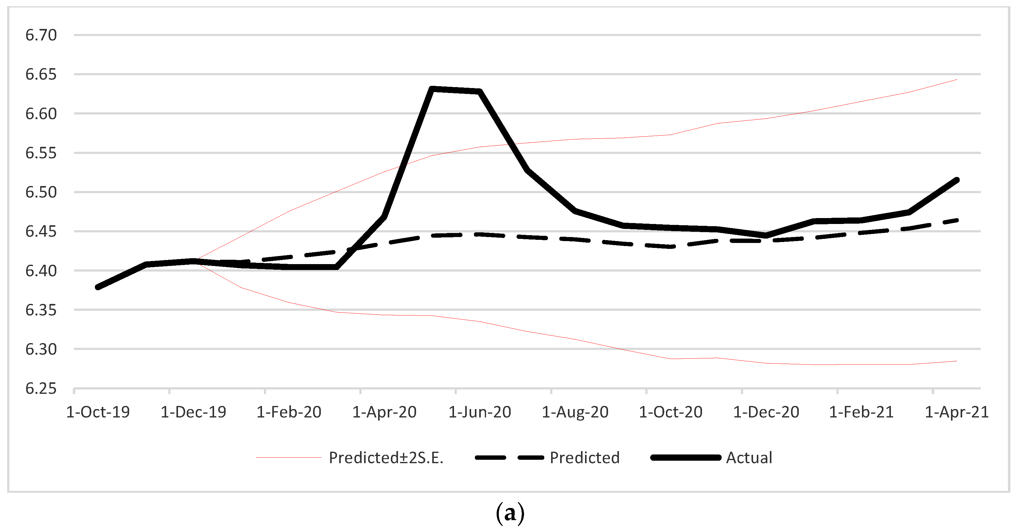
The empirical results show that there is asymmetric adjustment in speeds of prices in the U.S. beef supply chain. To measure the magnitude of price adjustment, we employ historical decomposition graphs. These graphs allow us to visualize the short-run dynamic effects of the COVID-19 shock on the prices in the neighborhood of the event, i.e., the COVID-19 shock. Figure 3a–c provides the historical decomposition graphs of the three price series for 15 months of the forecast horizon. We assumed the initial impact of COVID-19 on the prices started in March 2020, the beginning date of the spread of COVID-19, when the official policy responses and decisions took stage. Before April 2020, the actual and predicted data show almost the same patterns. However, we start to see significant differences between actual and predicted prices after that period. The historical decomposition graphs of predicted prices show positive changes for the retail and wholesale prices, but a negative impact for the farm level prices.
The historical decomposition graph of the wholesale prices (Figure 3) that include the impact of the shock, presents a wide departure of actual prices occurring immediately in April 2020 and continuing until July 2020. The maximum deviation from the predicted value is almost 10% in May 2020. The wholesale prices approach their predicted levels after 4 months.
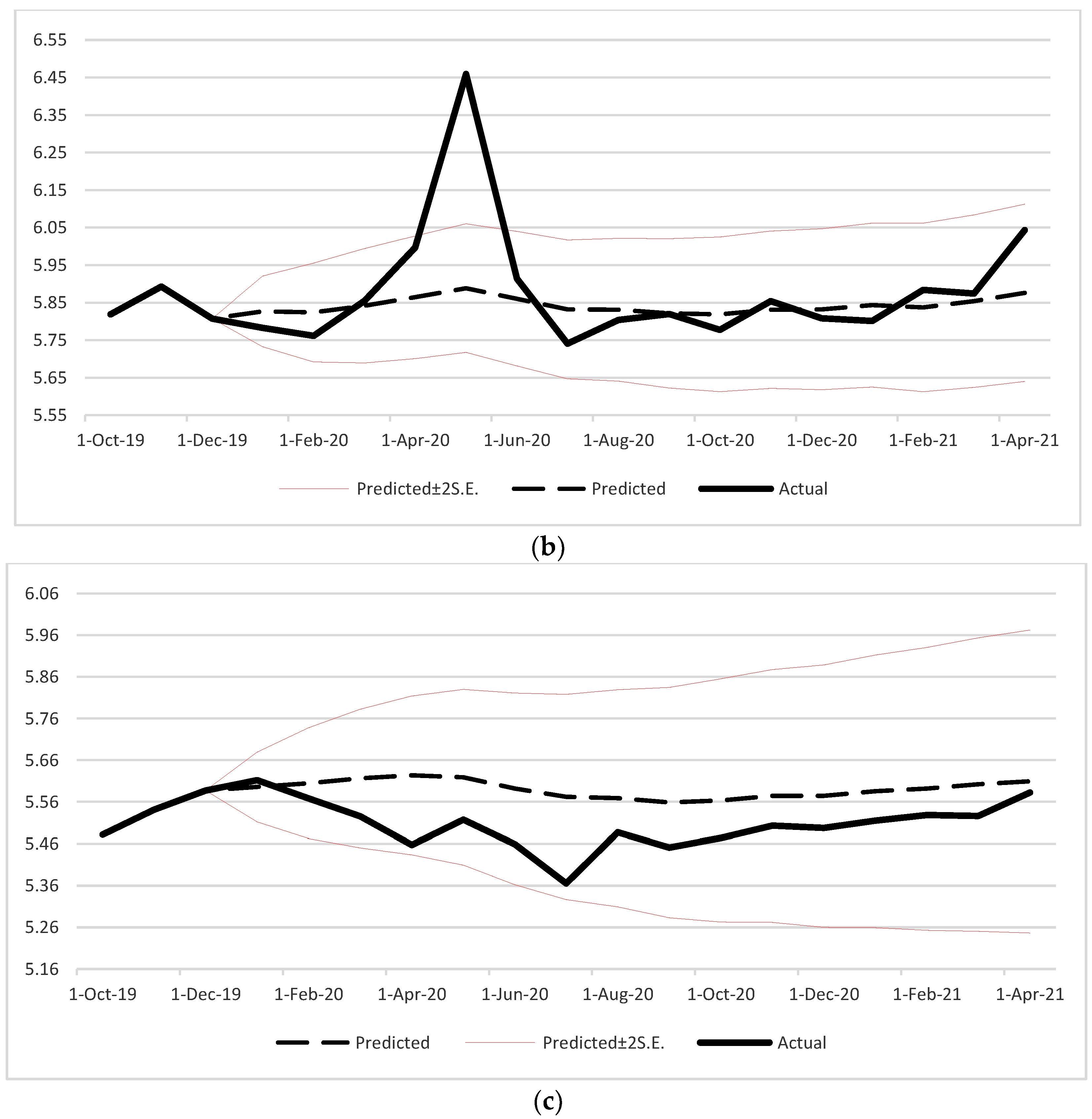
The historical decomposition graph of the retail prices also shows a positive change with divergence of actual prices starting in April 2020 and continuing until August 2020. The maximum deviation from predicted value is almost 3% in May 2020. The adjustment process of actual prices takes about 6 months to converge to the predicted price values. However, actual prices stay slightly above the predicted values after 6 months. These results, consistent with the results for speeds of adjustment, indicate a differential impacts of COVID-19 on wholesalers and retailers.
We observe more severe differential impact when analyzing the historical decomposition graph for the farm prices. As mentioned earlier, the only negative price effect due to the COVID-19 shock is on farm prices. Negative divergence of actual prices starts in April 2020 and ends by July 2020. The maximum deviation from predicted value is almost −4% in July 2020. These results clearly imply that in the short run, an exogenous COVID-19 shock on the U.S. beef sector impacted cattle producers negatively, while it positively affected packers and retailers. Although initial time of the shock is similar at all stages, impacted periods differ for each price. The magnitudes of price effects are substantially different for the three price series, resulting in widening the producer-retail price spreads.
5. Discussion
The results in Table 7 show that in case of the COVID-19 shock, wholesale prices adjusted more quickly than both farm (threefold) and retail prices (tenfold). It suggests that wholesale prices were more flexible than retail and farm prices in order to restore to the long run equilibrium with the COVID-19 shock. This conclusion is consistent with the results of Saghaian [35] and Darbandi and Saghaian [36] who used a similar methodology. However, it contradicts Goodwin and Holt [27] whose results showed a symmetric adjustment. Ramsey et al. [37] also found an asymmetric relation between retail and wholesale prices, but the speed of adjustment for retail prices was larger, having a higher speed of adjustment compared to the wholesale prices.
The economic literature accounts for a variety of reasons for the asymmetric adjustment in the U.S. beef markets. Balagtas and Cooper [6] discussed the market power exercised by meatpackers during COVID-19 and concluded that meatpackers took advantage of their market power to increase price margins. Lusk et al. [49] present a detailed analysis of the farm-to-wholesale margins in their study and they also pointed to increasing profitability of meat packers and processors working with a reduced capacity during the COVID-19 pandemic. In addition to the market power, product heterogeneity, long-term contracts, and adjustments or menu costs are other reasons stated for the existence of asymmetric price adjustment along the U.S. beef supply chain [27,35,50].
Results provided by historical decomposition graphs confirm an asymmetry in the magnitude in the U.S. beef prices. The outcomes of the event study in Ramsey et al. [37] also detected similar results for retail and wholesale prices and they cited the supply shortage during the pandemic as a reason for price spikes during April and May 2020 as we stated early. They defined these shocks as transitory and pointed out that the transition period is 1 to 3 months; our results found 4 to 6 months. Although we observe some minor differences between actual and predicted prices that imply price stickiness and incomplete price transmission after the shock period for some of the price levels, it can be said that U.S. beef markets are resilient enough to absorb the shocks and return to their pre-shock patterns in 4 to 6 months. Another major point is that farmers are the only and most adversely impacted economic actors in the U.S. beef supply chain during the COVID-19 shock. This outcome rationalizes the base for policy makers to prioritize farmers in support policies during similar crisis.
6. Conclusions and Policy Implications
The U.S. beef industry with its significant domestic production, processing, and international trade is one of the most important agricultural industries and thus, has drawn a considerable amount of attention from research institutions and academia. In addition to its economic value, beef is also an indispensable nutrition in the American diet. Due to its size and economic impact alongside with the federal and state level supports, any structural change in the production and market efficiency adds to the importance of price discovery and price adjustments in the beef sector.
This study proposed a methodology to investigate how the COVID-19 shock impacted the U.S. beef supply chain and examined whether dynamic price relations among the retailers, wholesalers, and farmers changed with this historical shock. We assumed that the actual shock period started in March of 2020 after the spread of COVID-19 started and related policy reactions in U.S were initiated. We employed contemporary time-series techniques in a VEC model augmented with structural breaks to measure the speeds of price adjustments. We utilized historical decomposition graphs to estimate the magnitude of price adjustments across the supply chain caused by the shock with monthly prices for the period from January 1970 to April 2021.
The empirical results add several contributions to the current literature, and provide a base for strategic agribusiness reactions for similar crisis. First, in this study, we evaluated the capability of markets to recover after an event such as the COVID-19 shock. We observed that U.S. beef markets are resilient enough to absorb the shock and return to their pre-shock patterns in 4 to 6 months. To obtain accurate results, we incorporated structural breaks into the model estimation of the dynamics of price adjustments in the U.S. beef markets. We detected four structural breaks in the price relations from farm to the retail level and found that the direction of price relationships are from farmers to wholesalers, to retailers in our dataset. Furthermore, the VEC model results show that there is an asymmetry in the speeds of price adjustments during the COVID-19 shock. The wholesale prices adjusted more quickly than farm (threefold) and retail prices (tenfold). That suggests higher flexibility of wholesale prices compared to the retail and farm prices, when prices restore to the long run equilibrium. These results have welfare and policy implications for the U.S. beef industry.
In addition, historical decomposition graphs show the existence of asymmetry in the magnitude of the price adjustments. This is consistent with the differential speeds of adjustments discovered. The impact causes retail and wholesale prices to be higher than their predicted values. That is, price spreads are widened due to the COVID-19 shock in favor of wholesalers and retailers. Hence, the shock has adversely affected the consumers in the U.S. beef marketing chain.
Meanwhile farm prices are lower than their predicted values due to the COVID-19 shock. That has an important agribusiness implication for the farmers in the U.S. beef supply chain. This study concludes that beef producers’ incomes are highly adversely impacted because of the shock and should be prioritized by policy makers during similar crisis such as COVID-19.
Author Contributions
E.E. has the primary role in this manuscript. He is responsible for collecting the data, modeling of the data, and drafting the manuscript. S.H.S.’s contribution in the paper is revision of the draft manuscript, and guidance on modeling questions. All authors have read and agreed to the published version of the manuscript.
Funding
This research received no external funding.
Institutional Review Board Statement
Not applicable.
Informed Consent Statement
Not applicable.
Data Availability Statement
The data is available upon request.
Acknowledgments
The authors acknowledge the support from the USDA, National Institute of Food and Agriculture, Hatch project No. KY004052, under accession number 1012994.
Conflicts of Interest
The authors declare no conflict of interest.
References
- NIAID. Coronaviruses. Available online: https://www.niaid.nih.gov/diseases-conditions/coronaviruses (accessed on 16 February 2022).
- USDA; FAS. Livestock and Poultry: World Markets and Trade. Washington, DC, USA, 2022. Available online: https://www.fas.usda.gov/data/livestock-and-poultry-world-markets-and-trade (accessed on 24 March 2022).
- USDA; ERS. Statistics & Information. Available online: https://www.ers.usda.gov/topics/animal-products/cattle-beef/statistics-information/ (accessed on 24 March 2022).
- USDA; ERS. Sector at a Glance. Available online: https://www.ers.usda.gov/topics/animal-products/cattle-beef/sector-at-a-glance/ (accessed on 24 March 2022).
- English, L.; Popp, J. Economic Contributions of the US Beef Industry. Presented at the National Cattlemen’s Beef Association Meeting, 16–17 November 2020; Available online: https://economic-impact-of-ag.uada.edu/files/2017/05/5-Popp-English_Economic-Contributions-of-the-US-Beef-Industry.pdf (accessed on 27 March 2022).
- Balagtas, J.V.; Cooper, J. The Impact of COVID-19 on United States Meat and Livestock Markets. AAEA Choices Mag. 2021, 36, 1–10. [Google Scholar]
- Bunge, J. Coronavirus Hits Meat Plants as Some Workers Get Sick, Others Stay Home. Available online: https://www.wsj.com/articles/coronavirus-hits-meat-plants-as-some-workers-get-sick-others-stay-home-11586196511 (accessed on 16 February 2022).
- Cowley, C. COVID-19 Disruptions in the U.S. Meat Supply Chain. Available online: https://www.kansascityfed.org/agriculture/ag-outlooks/COVID-19-US-Meat-Supply-Chain/ (accessed on 16 February 2022).
- Baldwin, R.; di Mauro, B.W. Economics in the Time of COVID-19; CEPR Press: London, UK, 2020. [Google Scholar]
- Bairoliya, N.; İmrohoroğlu, A. Macroeconomic Consequences of Stay-at-Home Policies during the COVID-19 Pandemic. Covid Econ. 2020, 13, 71–90. [Google Scholar]
- Laborde, D.; Martin, W.; Vos, R. Impacts of COVID-19 on Global Poverty, Food Security, and Diets: Insights from Global Model Scenario Analysis. Agric. Econ. 2021, 52, 375–390. [Google Scholar] [CrossRef] [PubMed]
- Beckman, J.; Countryman, A.M. The Importance of Agriculture in the Economy: Impacts from COVID-19. Am. J. Agric. Econ. 2021, 103, 1595–1611. [Google Scholar] [CrossRef]
- Thorbecke, W. The Impact of the COVID-19 Pandemic on the U.S. Economy: Evidence from the Stock Market. J. Risk Financ. Manag. 2020, 13, 233. [Google Scholar] [CrossRef]
- Swinnen, J.; Vos, R. COVID-19 and Impacts on Global Food Systems and Household Welfare: Introduction to a Special Issue. Agric. Econ. 2021, 52, 365–374. [Google Scholar] [CrossRef]
- Poudel, B.P.; Poudel, M.R.; Gautam, A.; Phuyal, S.; Tiwari, C.K.; Bashyal, N.; Bashyal, S. COVID-19 and Its Global Impact on Food and Agriculture. J. Biol. Today’s World 2020, 9, 221. [Google Scholar]
- Barman, A.; Das, R.; De, P.K. Impact of COVID-19 in Food Supply Chain: Disruptions and Recovery Strategy. Curr. Res. Behav. Sci. 2021, 2, 100017. [Google Scholar] [CrossRef]
- Van Hoyweghen, K.; Fabry, A.; Feyaerts, H.; Wade, I.; Maertens, M. Resilience of Global and Local Value Chains to the COVID-19 Pandemic: Survey Evidence from Vegetable Value Chains in Senegal. Agric. Econ. 2021, 52, 423–440. [Google Scholar] [CrossRef]
- Guo, J.; Tanaka, T. The Effectiveness of Self-Sufficiency Policy: International Price Transmissions in Beef Markets. Sustainability 2020, 12, 6073. [Google Scholar] [CrossRef]
- Almadani, M.I.; Weeks, P.; Deblitz, C. COVID-19 Influence on Developments in the Global Beef and Sheep Sectors. Ruminants 2021, 2, 27–53. [Google Scholar] [CrossRef]
- Zamani, O.; Bittmann, T.; Loy, J.-P. Food Markets Performance under the COVID-19 Pandemic: A Case Study of Meat Industry in Iran. Appl. Econ. Lett. 2022, 1–6. [Google Scholar] [CrossRef]
- Hayes, D.J.; Schulz, L.L.; Hart, C.E.; Jacobs, K.L. A Descriptive Analysis of the COVID-19 Impacts on U.S. Pork, Turkey, and Egg Markets. Agribusiness 2021, 37, 122–141. [Google Scholar] [CrossRef]
- Siche, R. What Is the Impact of COVID-19 Disease on Agriculture? Sci. Agropecu. 2020, 11, 3–6. [Google Scholar] [CrossRef] [Green Version]
- Mead, D.; Ransom, K.; Reed, S.B.; Sager, S. The Impact of the COVID-19 Pandemic on Food Price Indexes and Data Collection. Mon. Labor Rev. 2020, 1–13. [Google Scholar] [CrossRef]
- Meyer, J.; von Cramon-Taubadel, S. Asymmetric Price Transmission: A Survey. J. Agric. Econ. 2004, 55, 581–611. [Google Scholar] [CrossRef] [Green Version]
- Vavra, P.; Goodwin, B.K. Paper 3—Analysis of price transmission along the food chain. In OECD Food, Agriculture and Fisheries Papers; OECD Publishing: Paris, France, 2005. [Google Scholar]
- Lloyd, T. Forty Years of Price Transmission Research in the Food Industry: Insights, Challenges and Prospects. J. Agric. Econ. 2017, 68, 3–21. [Google Scholar] [CrossRef] [Green Version]
- Goodwin, B.K.; Holt, M.T. Price Transmission and Asymmetric Adjustment in the U.S. Beef Sector. Am. J. Agric. Econ. 1999, 81, 630–637. [Google Scholar] [CrossRef]
- Rojas, C.; Andino, A.; Purcell, W. Retailers’ Response to Wholesale Price Changes: New Evidence from Scanner-Based Quantity-Weighted Beef Prices. Agribusiness 2008, 24, 1–15. [Google Scholar] [CrossRef] [Green Version]
- Boetel, B.L.; Liu, D.J. Estimating Structural Changes in the Vertical Price Relationships in U.S. Beef and Pork Markets. J. Agric. Resour. Econ. 2010, 35, 228–244. [Google Scholar] [CrossRef]
- Surathkal, P.; Chung, C.; Han, S. Asymmetric adjustments in vertical price transmission in the US beef sector: Testing for differences among product cuts and quality grade. In Proceedings of the 2014 Agricultural and Applied Economics Association Annual Meeting, Minneapolis, MI, USA, 27–29 July 2014. [Google Scholar] [CrossRef]
- Emmanouilides, C.J.; Fousekis, P. Vertical Price Dependence Structures: Copula-Based Evidence from the Beef Supply Chain in the USA. Eur. Rev. Agric. Econ. 2015, 42, 77–97. [Google Scholar] [CrossRef] [Green Version]
- Fousekis, P.; Katrakilidis, C.; Trachanas, E. Vertical Price Transmission in the US Beef Sector: Evidence from the Nonlinear ARDL Model. Econ. Model. 2016, 52, 499–506. [Google Scholar] [CrossRef]
- Pozo, V.F.; Bachmeier, L.J.; Schroeder, T.C. Are There Price Asymmetries in the U.S. Beef Market? J. Commod. Mark. 2021, 21, 100–127. [Google Scholar] [CrossRef]
- Livanis, G.T.; Moss, C.B. Price transmission and food scares in the U.S. beef sector. In Proceedings of the 2005 American Agricultural Economics Association Annual Meeting, Providence, RI, USA, 24–27 July 2005. [Google Scholar]
- Saghaian, S.H. Beef Safety Shocks and Dynamics of Vertical Price Adjustment: The Case of BSE Discovery in the U.S. Beef Sector. Agribusiness 2007, 23, 333–348. [Google Scholar] [CrossRef]
- Darbandi, E.; Saghaian, S.H. Vertical Price Transmission in the U.S. Beef Markets with a Focus on the Great Recession. J. Agribus. 2016, 34, 91–110. [Google Scholar]
- Ramsey, A.F.; Goodwin, B.K.; Hahn, W.F.; Holt, M.T. Impacts of COVID-19 and Price Transmission in U.S. Meat Markets. Agric. Econ. 2021, 52, 441–458. [Google Scholar] [CrossRef] [PubMed]
- Engle, R.F.; Granger, C.W.J. Co-Integration and Error Correction: Representation, Estimation, and Testing. Econometrica 1987, 55, 251–276. [Google Scholar] [CrossRef]
- Johansen, S. Estimation and Hypothesis Testing of Cointegration Vectors in Gaussian Vector Autoregressive Models. Econometrica 1991, 59, 1551. [Google Scholar] [CrossRef]
- Dickey, D.A.; Fuller, W.A. Distribution of the Estimators for Autoregressive Time Series with a Unit Root. J. Am. Stat. Assoc. 1979, 74, 427–431. [Google Scholar] [CrossRef]
- Kwiatkowski, D.; Phillips, P.C.B.; Schmidt, P.; Shin, Y. Testing the Null Hypothesis of Stationarity against the Alternative of a Unit Root: How Sure Are We That Economic Time Series Have a Unit Root? J. Econom. 1992, 54, 159–178. [Google Scholar] [CrossRef]
- Özertan, G.; Saghaian, S.; Tekgüç, H. Market Power in the Poultry Sector in Turkey. Boğaziçi J. Rev. Soc. Econ. Adm. Stud. 2014, 28, 19–32. [Google Scholar] [CrossRef]
- Zivot, E.; Andrews, D.W.K. Further Evidence on the Great Crash, the Oil-Price Shock, and the Unit-Root Hypothesis. J. Bus. Econ. Stat. 1992, 10, 251. [Google Scholar] [CrossRef] [Green Version]
- Bai, J. Estimation of a Change Point in Multiple Regression Models. Rev. Econ. Stat. 1997, 79, 551–563. [Google Scholar] [CrossRef]
- Pala, A. Structural Breaks, Cointegration, and Causality by VECM Analysis of Crude Oil and Food Price. Int. J. Energy Econ. Policy 2013, 3, 238–246. [Google Scholar]
- Chopra, A.; Bessler, D.A. Impact of BSE and FMD on beef industry in U.K. In Proceedings of the NCR-134 Conference on Applied Commodity Price Analysis, Forecasting, and Market Risk Management, St. Louis, MO, USA, 18–19 April 2005. [Google Scholar]
- Estima. Regression Analysis of Time Series User’s Guide; Estima: Evaston, IL, USA, 2010. [Google Scholar]
- Bai, J.; Perron, P. Computation and Analysis of Multiple Structural Change Models. J. Appl. Econom. 2003, 18, 1–22. [Google Scholar] [CrossRef] [Green Version]
- Lusk, J.L.; Tonsor, G.T.; Schulz, L.L. Beef and Pork Marketing Margins and Price Spreads during COVID-19. Appl. Econ. Perspect. Policy 2021, 43, 4–23. [Google Scholar] [CrossRef]
- Zachariasse, L.C.; Bunte, F.H.J. How are farmers faring in the changing balance of power along the food chain? In Proceedings of the OECD-Conference on Changing Dimensions of the Food Economy: Exploring the Policy Issues, Hague, The Netherlands, 6–7 February 2003. [Google Scholar]
Figure 1.
U.S. beef prices (Cents per pound).

Figure 2.
U.S. beef price spreads (Cents per pound-Averages of January 2016–April 2021).

Figure 3.
Historical Decomposition Graphs. (a) Retail prices. (b) Wholesale prices. (c) Farm prices.
Figure 3.
Historical Decomposition Graphs. (a) Retail prices. (b) Wholesale prices. (c) Farm prices.


Table 1.
Summary statistics.
| Level | Retail | Wholesale | Farm |
| Mean | 330.00 | 198.48 | 166.95 |
| Median | 283.85 | 176.00 | 150.85 |
| Maximum | 758.51 | 638.56 | 367.02 |
| Minimum | 98.00 | 71.50 | 58.80 |
| Std. Dev. | 152.98 | 78.10 | 63.25 |
| Observations | 616 | 616 | 616 |
| Log | Retail | Wholesale | Farm |
| Mean | 5.69 | 5.22 | 5.05 |
| Median | 5.65 | 5.17 | 5.02 |
| Maximum | 6.63 | 6.46 | 5.91 |
| Minimum | 4.58 | 4.26 | 4.07 |
| Std. Dev. | 0.49 | 0.39 | 0.38 |
| Observations | 616 | 616 | 616 |
Table 2.
ADF and KPSS test results.
| ADF t-Statistic (BIC Lag) | Levels Intercept | Levels Intercept and Trend | 1st Difference Intercept | 1st Difference Intercept and Trend | Result |
| retail | −1.30 (2) | −3.01 (2) | −17.73 * (1) | −17.74 * (1) | I(1) |
| wholesale | −1.45 (4) | −3.40 *** (4) | −16.43 * (3) | −16.42 * (3) | I(0) |
| farm | −1.99 (4) | −3.24 *** (4) | −16.24 * (3) | −16.25 * (3) | I(0) |
| KPSS t-Statistic | Levels Intercept | Levels Intercept and Trend | 1st Difference Intercept | 1st Difference Intercept and Trend | Result |
| retail | 3.11 * | 0.25 * | 0.14 | 0.08 | I(1) |
| wholesale | 2.87 * | 0.26 * | 0.104 | 0.103 | I(1) |
| farm | 2.74 * | 0.214 | 0.12 | 0.07 | I(0) |
Note: Critical values are −3.44, −2.86, and −2.57 for levels and intercept and −3.97, −3.41, and −3.13 for levels, intercept, and trend, respectively, at 1%, 5% and 10% for ADF. Critical values are 0.74, 0.46, and 0.35 for levels and intercept and 0.22, 0.15, and 0.12 for levels, intercept, and trend, respectively, at 1%, 5% and 10% for KPSS. * and *** indicate rejection of the null hypothesis at 1% and 10% levels, respectively.
Table 3.
Zivot-Andrews unit root test allowing for one structural break.
| t-Statistic (BIC Lag) Break Point | Levels Intercept | Levels Intercept and Trend | 1st Difference Intercept | 1st Difference Intercept and Trend | Result | |
|---|---|---|---|---|---|---|
| Intercept | Intercept and Trend | |||||
| retail | −3.83 (2) 1993m6 | −3.96 (2) 1982m7 | −17.98 * (1) 1979m6 | −18.07 * (1) 1979m6 | I(1) | I(1) |
| wholesale | −4.76 (4) 1993m6 | −4.70 (4) 1993m6 | −16.55 * (3) 1979m6 | −16.57 * (3) 1979m6 | I(1) | I(1) |
| farm | −4.27 (4) 1993m6 | −4.18 (4) 1993m6 | −16.37 * (3) 1999m1 | −16.42 * (3) 2015m6 | I(1) | I(1) |
Note: * indicates rejection of the null hypothesis at 5%. Critical values are −4.80 and −5.08 for intercept and intercept and trend, respectively.
Table 4.
Granger causality test results.
| Null Hypothesis | F-Statistic |
|---|---|
| Farm price does not granger cause wholesale price | 19.84 * |
| Wholesale price does not granger cause farm price | 1.43 |
| Wholesale price does not granger cause retail price | 82.08 * |
| Retail price does not granger cause wholesale price | 17.20 * |
| Farm price does not granger cause retail price | 76.55 * |
| Retail price does not granger cause farm price | 23.19 * |
Note: * 1% significance level.
Table 5.
L + 1 vs. L sequentially determined breaks.
| Break Test | F-Statistics | Critical Value ** | Number of Breaks | Dates |
|---|---|---|---|---|
| 0 vs. 1 * | 36.92 | 13.98 | 1 | 1980M11 |
| 1 vs. 2 * | 29.56 | 15.72 | 2 | 1993M07 |
| 2 vs. 3 * | 21.86 | 16.83 | 3 | 2001M05 |
| 3 vs. 4 * | 19.52 | 17.61 | 4 | 2013M09 |
| 4 vs. 5 | 0.00 | 18.14 | 4 |
Note: * indicates rejection of the null hypothesis at 5%. ** Bai-Perron (2003) critical values.
Table 6.
Johansen cointegration test results.
| Null Hypothesis a | Trace Statistics | 5% Critical Value | Eigenvalue |
|---|---|---|---|
| r = 0 * | 146.12 | 21.13 | 0.00 |
| r ≤ 1 * | 39.14 | 14.26 | 0.00 |
| r ≤ 2 | 0.48 | 3.84 | 0.49 |
Note: a: r is the cointegrating rank, * rejection of the null hypothesis at the 5% level.
Table 7.
The empirical estimates of speeds of adjustment and diagnostics.
| Variable | |||
|---|---|---|---|
| Speeds of adjustment | −0.021 ** | 0.206 * | 0.074 * |
| Model diagnostics | |||
| R2 | 0.38 | 0.23 | 0.17 |
| AIC | −5.37 | −3.25 | −3.47 |
| SIC | −5.23 | −3.10 | −3.33 |
Note: * 1% and ** 5% significance level.
Publisher’s Note: MDPI stays neutral with regard to jurisdictional claims in published maps and institutional affiliations. |
© 2022 by the authors. Licensee MDPI, Basel, Switzerland. This article is an open access article distributed under the terms and conditions of the Creative Commons Attribution (CC BY) license (https://creativecommons.org/licenses/by/4.0/).
Share and Cite
MDPI and ACS Style
Erol, E.; Saghaian, S.H. The COVID-19 Pandemic and Dynamics of Price Adjustment in the U.S. Beef Sector. Sustainability 2022, 14, 4391. https://doi.org/10.3390/su14084391
AMA Style
Erol E, Saghaian SH. The COVID-19 Pandemic and Dynamics of Price Adjustment in the U.S. Beef Sector. Sustainability. 2022; 14(8):4391. https://doi.org/10.3390/su14084391
Chicago/Turabian StyleErol, Erdal, and Sayed H. Saghaian. 2022. "The COVID-19 Pandemic and Dynamics of Price Adjustment in the U.S. Beef Sector" Sustainability 14, no. 8: 4391. https://doi.org/10.3390/su14084391
Note that from the first issue of 2016, this journal uses article numbers instead of page numbers. See further details here.