
Pattern Formation Induced by Fuzzy Fractional-Order Model of COVID-19
by
 , ,
, ,
Abeer S. Alnahdi
1,† ,
,
Ramsha Shafqat
2,*,†,
Azmat Ullah Khan Niazi
2,† and
Mdi Begum Jeelani
1,*,† 1
Department of Mathematics and Statistics, College of Science, Imam Mohammad Ibn Saud Islamic University, Riyadh 11564, Saudi Arabia
2
Department of Mathematics and Statistics, The University of Lahore, Sargodha 40100, Pakistan
*
Authors to whom correspondence should be addressed.
†
These authors contributed equally to this work.
Axioms 2022, 11(7), 313; https://doi.org/10.3390/axioms11070313
Submission received: 30 May 2022
/
Revised: 14 June 2022
/
Accepted: 23 June 2022
/
Published: 27 June 2022
(This article belongs to the Special Issue Calculus of Variations, Optimal Control, and Mathematical Biology: A Themed Issue Dedicated to Professor Delfim F. M. Torres on the Occasion of His 50th Birthday)
Abstract
:A novel coronavirus infection system is established for the analytical and computational aspects of this study, using a fuzzy fractional evolution equation (FFEE) stated in Caputo’s sense for order (1,2). It is constructed using the FFEE formulated in Caputo’s meaning. The model consist of six components illustrating the coronavirus outbreak, involving the susceptible people , the exposed population , total infected strength , asymptotically infected population , total number of humans recovered , and reservoir . Numerical results using the fuzzy Laplace approach in combination with the Adomian decomposition transform are developed to better understand the dynamical structures of the physical behavior of COVID-19. For the controlling model, such behavior on the generic characteristics of RNA in COVID-19 is also examined. The findings show that the proposed technique of addressing the uncertainty issue in a pandemic situation is effective.
Keywords:
approximation solution; fuzzy number; fuzzy fractional order derivative; coronavirus infection system; Adomian decomposition methodMSC:
26A33; 34K371. Introduction
Recently, the entire world has been afflicted by a novel coronavirus pandemic known as the “novel coronavirus 2019”, abbreviated as “nCOVID-19”, which was initially reported in Wuhan, central China [1]. It has been discovered that nCOVID-19 is spread from animal to human; several afflicted people claimed to have contracted the virus after visiting a local fish and wild animal market in Wuhan on 28 November [2]. Following that, other researchers confirmed that transmission can also occur from one person to another [3]. According to World Health Organization data, the number of reported laboratory-confirmed human infections in 187 countries, territories, or places around the world reached 292,142 on 21 March 2020, with 12,784 mortality cases [4]. The death rate was as high as 0.0666 in some nations, such as Italy and Spain. This confirms the severity and high infectivity of nCOVID-19. Most patients infected with nCOVID-19 will have mild to moderate respiratory symptoms, such as shortness of breath, low fever, nausea, cough, and other symptoms. Other symptoms have been described, including gastroenteritis and neurological illnesses of varying severity [5]. nCOVID-19 is primarily transmitted by droplets from the nose when an infected person coughs or sneezes. A person is in danger of catching the virus if he or she inhales droplets from infected people in the air. As a result, avoiding meetings and contacting other individuals is the greatest approach to avoid contracting the virus.
To manage people flow and movement, Wuhan has been shut down by the Chinese government, and they have decreased or restricted the transportation system of the country, including airplanes, trains, buses, and private cars, among other things. People have had to stay at home and have their body temperature taken every day. If they have to go outside, they are advised to wear respirators. With the spread of nCOVID-19 around the world, more governments have entered the antivirus fight in the footsteps of the Chinese government. It was reported that an increasing number of governments have begun to issue restrictions prohibiting international travel, as well as closing schools, shopping malls, and businesses. The nCOVID-19 pandemic has caused significant economic loss throughout the world, as well as huge hardship for country administrations and even all human beings. A large number of doctors and researchers also dedicated themselves to the anti-pandemic fight and conducted research based on their knowledge. They studied nCOVID-19 from a variety of perspectives, including microbiology, virology, sociology, veterinary sciences, infectious diseases, public environmental occupational health, political economy, media studies, and so on. The main countries in nCOVID-19 research include China, the United States, and Korea, as a result of the virus’s early epidemic, which prompted them to begin relevant research right away. The origins of nCOVID-19 were investigated by a group of scientists. Initially, bats were thought to be the source of nCOVID-19, which is comparable to SARS (severe acute respiratory syndrome), a worldwide epidemic that began in China and other parts of the world in 2003 [6,7].
Following that, some studies linked nCOVID-19 to the 2012 pandemics of SARS and MERS (Middle East respiratory syndrome) to show that there are lessons to be learned from the two pandemics. SARS-COVID, MERS-COVID, and nCOVID-19 all belong to SARS-COVID, according to Lu [8] and belong to the same family of Betacoronaviruses. Previous studies, according to Zhou, suggest that nCOVID-19 has a significant degree of resemblance to SARS-COVID, and, as evidenced by [9], has the same predicted cell entry mechanism and human cell receptor use based on full-length genome phylogenetic research. Xiaolong and Mose also analyzed the high RBD (receptor binding domain) identity between nCOVID-19 and SARS-COVID, and proposed that the SARS-COVID specific human antibody, CR3022, might bind potently to the virus. nCOVID-19 RBD has a KD of 6.3 nM, indicating that the difference within the RBD is 6.3 nM. SARS-COVID and nCOVID-19 have a significant impact on neutralizing antibody cross-reactivity, which is still needed to produce novel monoclonal antibodies that bind selectively to nCOVID-19 RBD [10]. Syed et al. determined SARS-COVID-derived B lymphocyte epitopes and T-cell epitopes experimentally based on previous studies on SARS-COVID immunological systems and structures and discovered that they are similar and contain no mutation within the available nCOVID-19 sequences, which is critical for narrowing down the hunt for potent targets for an efficient vaccine against the nCOVID-19. Some researchers are concentrating on the transmission and identification of the nCOVID-19 virus in people. Human-to-human transmission is widely acknowledged as a factor in the rapid spread of illnesses. Ahmed said that viral strains from the area’s affected persons had been analyzed, but that there was a limited genetic difference, meaning that they all descended from a single ancestor [11]. Zhou, on the other hand, claimed that the sequences of the seven conserved viral replicase domains in ORF 1ab in nCOVID-19 and SARS-COVID [9] are 94.6 percent similar. Chaudhury et al. demonstrated that using accurate, physics-based energy functions, computational protein–protein docking can disclose the native-like, low-energy protein–protein complex from the unbound structures of two separate, interacting protein components [12]. In this paper, we attempt to mathematically examine the nCOVID-19 infection mechanism. The numerical findings are obtained using the fuzzy Laplace transform based on Adomian decomposition, which can be useful in understanding the dynamical structures of the physical behavior of nCOVID-19. In the form of nonlinear fractional order differential equations (FODEs), we define the system of six equations illustrating the coronavirus outbreak, involving susceptible people , the exposed population , total infected strength , asymptotically infected population , total number of humans recovered , and reservoir , which are listed in the following order [13]:
where is the birth rate, is the death rate of infected people, is the transmission coefficient, is the disease transmission coefficient, and is the transmissibility multiple. The symbols and signify the incubation period. The recovery rates of and are represented by and , respectively. and reflect the virus’s influence from and to , respectively, and indicates the virus’s elimination rate from . The parameters are included in Table 1 for convenience. In recent years, fuzzy calculus and FODEs [14,15,16,17] have been added to current calculus and DEs, respectively. Then, FODEs were expanded to fuzzy FODEs [18,19,20]. Many academics have researched FODEs and fuzzy integral equations in order to establish the existence–uniqueness theory of solutions [21,22,23,24,25,26]. It is extremely time consuming to compute more precise solutions to each fuzzy FODE when dealing with fuzzy FODEs. Mathematicians have put forth a lot of effort to solve fuzzy FODEs using various approaches, such as perturbation methods, integral transform methods, and spectral techniques [27,28,29,30,31,32]. Some researchers examined the stability of fuzzy DEs [33]. Niazi et al. [34], Iqbal et al. [35], Shafqat et al. [36] and Abuasbeh et al. [37] investigated the existence and uniqueness of the FFEE. Ahmad et al. [38] worked on Model (2), the fuzzy fractional-order model of the novel coronavirus as
Inspired by the above, Model (3) with a fuzzy fractional-order derivative by using mild solution is investigated here, with the uncertainty in initial data. For ,
associated to fuzzy initial condition, for ,
where is birth rate, is death rate of infected people, is transmission coefficient, is the disease transmission coefficient, and is the transmissibility multiple. The symbols and signify the incubation period. The recovery rates of and are represented by and , respectively. and reflect the virus’s influence from and to , respectively, and indicates the virus’s elimination rate from .
We use fuzzy fractional-order model of order (1, 2) by using a fuzzy mild solution of the novel coronavirus with nonlocal conditions. Owing to it, our model’s graphs are more accurate. The theory of fuzzy sets continues to gain scholars’ attention because of its huge range of applications in domains such as engineering, mechanics, robotics, electrical, control, thermal systems, and signal processing. In light of the foregoing arguments and to meet the current uncertain scenario, based on fuzzy fractional calculus, we suggested a new coronavirus infection strategy. We ensure that the proposed model is closer to the true behavior of a system growing the basic properties of RNA in COVID-19 by researching it, which also improves the physical behavior of such an infection system. Our major goal is to obtain the existence–uniqueness result of a COVID-19 model of order (1, 2). Applying mild solutions to this COVID-19 model becomes more complicated. However, via rigorous analysis, we show that the suggested function deduces a novel representation of solution operators and then provides a new idea of mild solutions. As a result, the research of system (3) differs greatly from earlier studies on the COVID-19 model. The other section of this paper is as follows. Section 2 discusses the definitions. Section 3 introduces the existence–uniqueness of the solution to the succeeding fuzzy model. A general method is also shown here for using fuzzy Laplace transform to determine the solution of the examined system. In Section 4, numerical results and discussion are presented. Finally, in Section 5, a conclusion is given.
2. Preliminaries
Definition 1
- (i)
- ρ is normal.
- (ii)
- ρ is upper semicontinuous on .
- (iii)
- ρ is convex.
- (iv)
- is compact.
Then, it is known as a fuzzy number.
Definition 2
Definition 3
([39,40]). Suppose is the parametric form of a fuzzy number ρ, where and the below properties are satisfied:
- (a)
- is left continuous, bounded, and increasing function over and right continuous at 0.
- (b)
- is left continuous, bounded, and increasing function over and right continuous at 0.
- (c)
Additionally, if , then θ is called a crisp number.
Definition 4
([30]). If a mapping and let and be two fuzzy numbers in their parametric form. The Hausdorff distance between ϱ and μ is defined as
In , the metric has the below properties:
- (i)
- for all ;
- (ii)
- for all ;
- (iii)
- for all ;
- (iv)
- is a complete metric space.
Definition 5
([30]). Let . If there exist such that then is said to be the H-difference of and , denoted by .
Definition 6
([30]). If be a fuzzy mapping. Then is called continuous if for any and a fixed value of , we have
whenever
Definition 7
([27,30]). Let φ be a continuous fuzzy function on , a fuzzy fractional integral in RL sense corresponding to ω is defined by
If , where and are the spaces of fuzzy continuous fractions and fuzzy Lebesgue integrable functions, respectively, then the fuzzy fractional integral is defined as
where
Definition 8
([30]). If a fuzzy fraction is such that and , then the fuzzy fractional Caputo’s derivative is defined as
where
whenever the integrals on the right-hand sides converge and .
Definition 9
([29,30,31]). Suppose ϕ is a continuous fuzzy-valued function. Assume that is an improper fuzzy Riemann-integrable on , then its fuzzy Laplace transform is
For , the parametric form of is represented by
Hence,
Theorem 1
([31]). If , then the Laplace transform of the fuzzy fractional derivative in Caputo’s form is given for and by
Theorem 2
(Schauder Fixed Point Theorem). Let be a Banach space and be compact, convex and nonempty. Any continuous operator has at least one fixed point.
3. Main Result
The existence–uniqueness of solutions to succeeding fuzzy fractional model (FFM) are examined in the following section, and we show how to discover a semi-analytic solution to model (3) using the fuzzy Laplace transform by using mild the solution.
3.1. Existence–Uniqueness
The existence–uniqueness of the succeeding FFM are addressed in this section using fixed point theory. Consider the right-hand side of Model (3):
where and are fuzzy functions. Thus, for , the model (3) is
with fuzzy initial conditions
Now applying a mild solution and using the initial conditions, we obtain
Let us define a Banach space as under the fuzzy norm:
On the nonlinear function , we add the following assumptions:
Assumption 1
(). There exists constant such that for each ,
Assumption 2
(). There exist constants such that
Theorem 3.
Under Assumption 2, the considered Model (5) has at least one solution.
Proof.
Suppose is a closed and convex fuzzy set, and is a mapping defined as
For any , we have
We obtain from the previous inequality, implying that the operator is bounded. The operator is then shown to be completely continuous. Allow to be such that , and then
We can see that the right-hand side of the inequality goes to zero as . Hence,
As a result, is an equicontinuous operator. The operator is entirely continuous according to the Arzela–Ascoli theorem, and it was previously bounded. As a result of Schauder’s fixed point theorem, System (5) has at least one solution. □
Theorem 4.
If , the investigated system (5) has a unique solution if Assumption 1 holds.
Proof.
Let , then
As a result, is a contraction. As a result, according to the Banach contraction theorem, System (5) has a single solution. □
3.2. Procedure for Solution
A general method is shown here for using the fuzzy Laplace transform to determine the solution of the examined system.
We have the fuzzy Laplace transform of (5) when we use beginning conditions:
The infinite series solution is
where and are Adomian polynomials that represent nonlinear terms. As a result, the final equation is
When we use the inverse Laplace transform, we obtain
We evaluate the first two terms of two terms of the series when comparing the terms on both sides:
We may find the other terms in the same way.
As a result, the examined system’s series solution is
4. Numerical Results and Discussion
We take a look at Table 1 that corresponds to the model’s parameters. Consider initial conditions for the proposed model (3).
We used the initial conditions and applied the proposed procedure to (3):
The second term of the series solution is
assume that
The series’ third term is now underway.
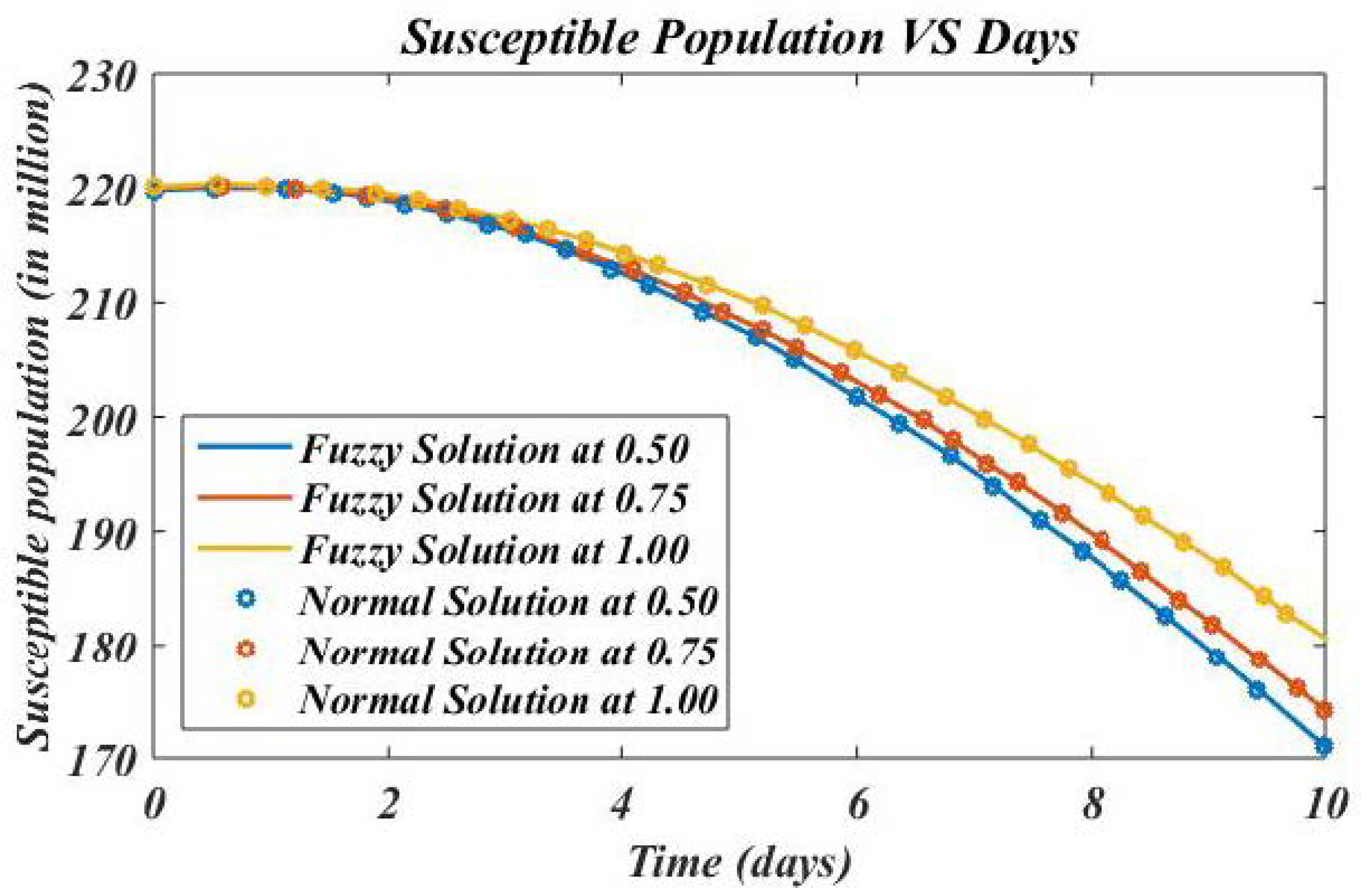
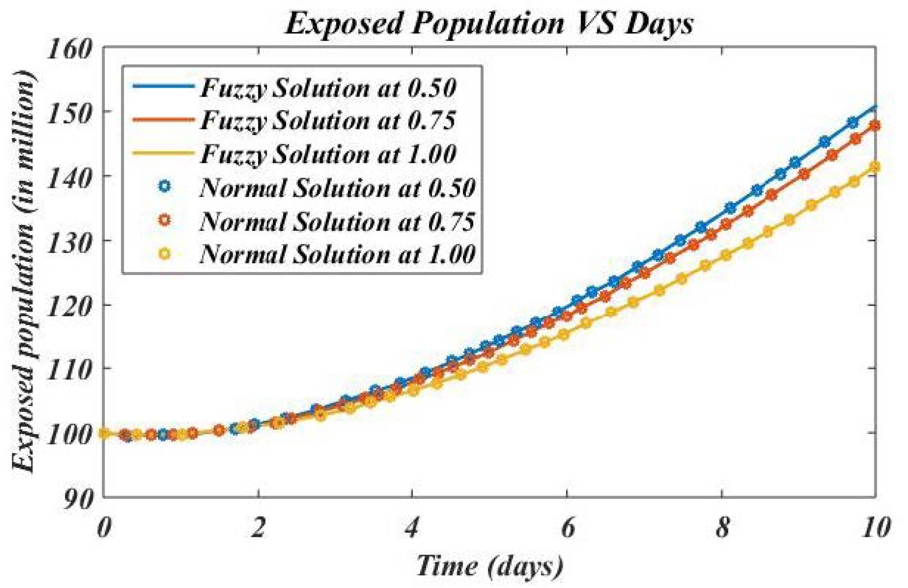
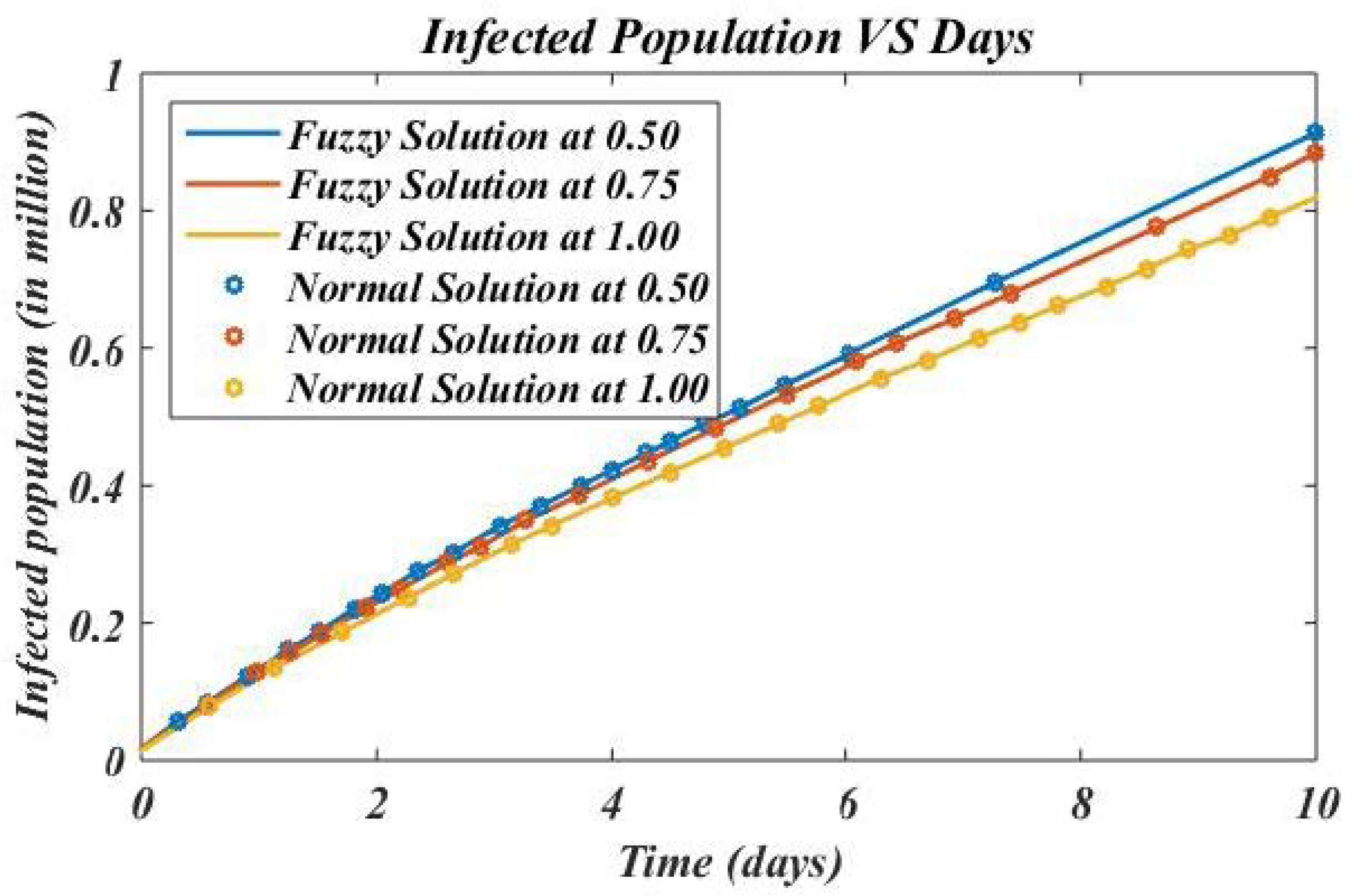
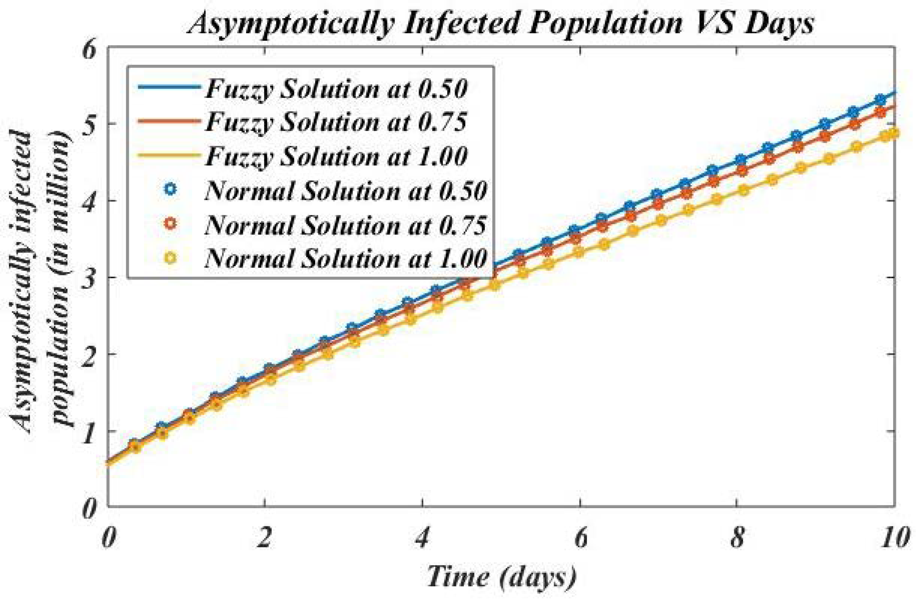
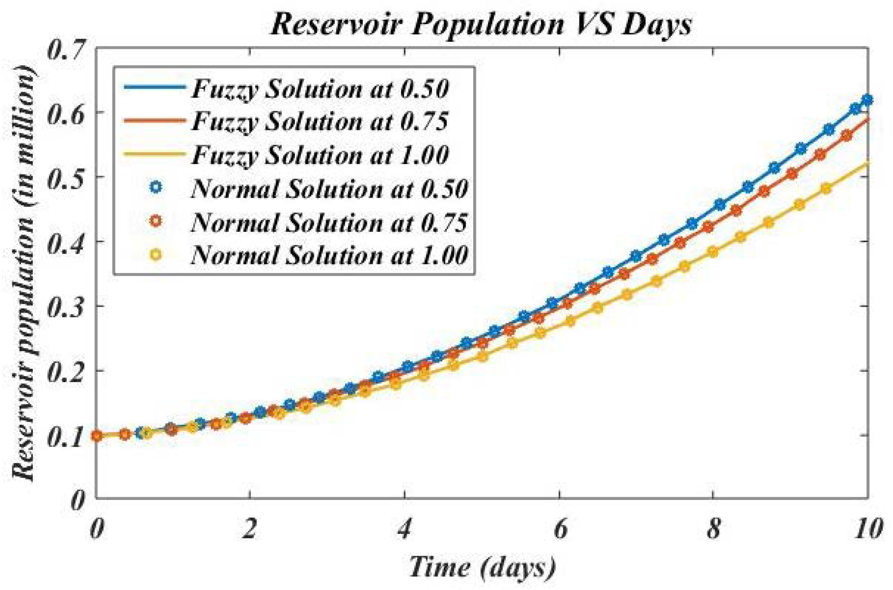
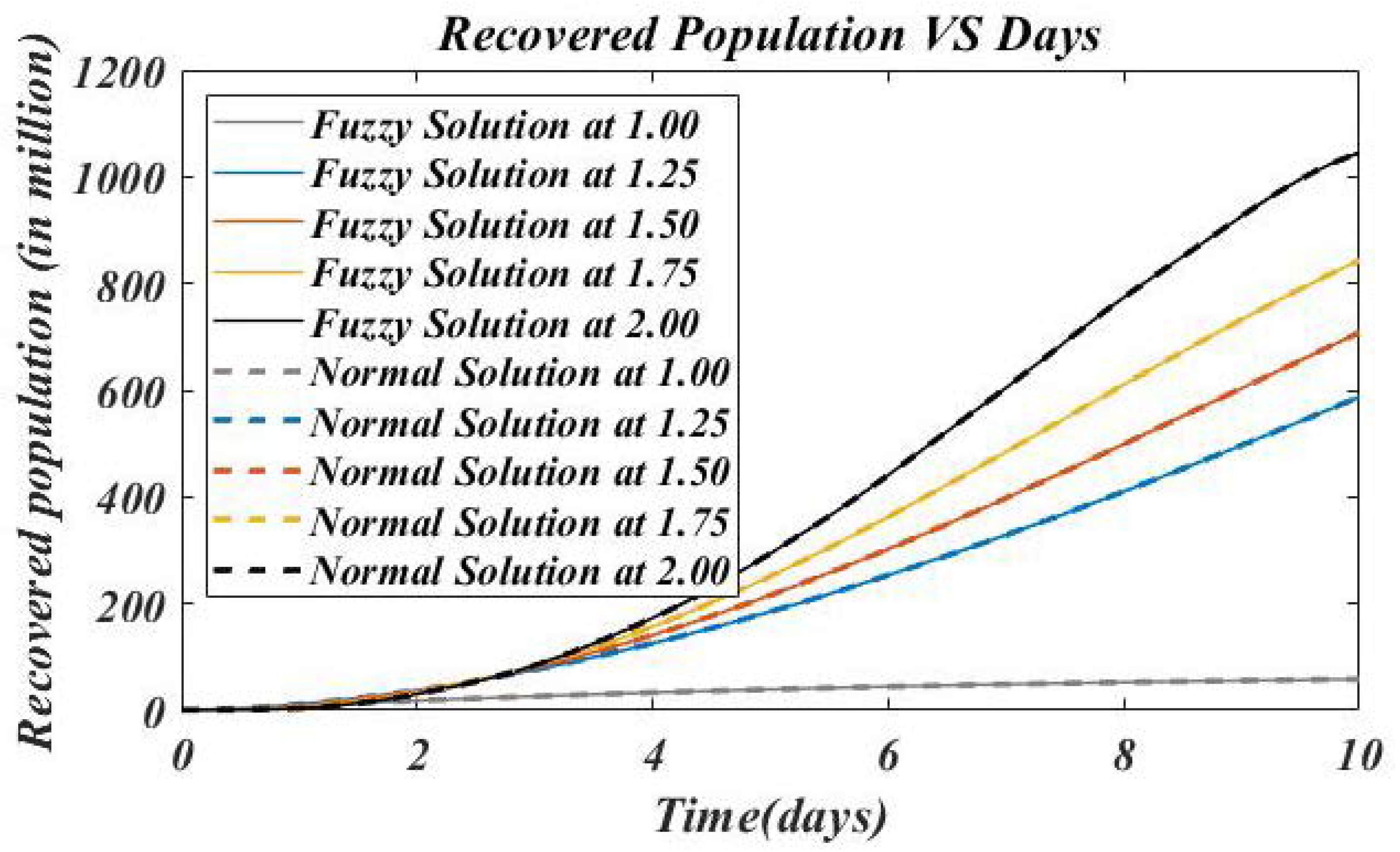
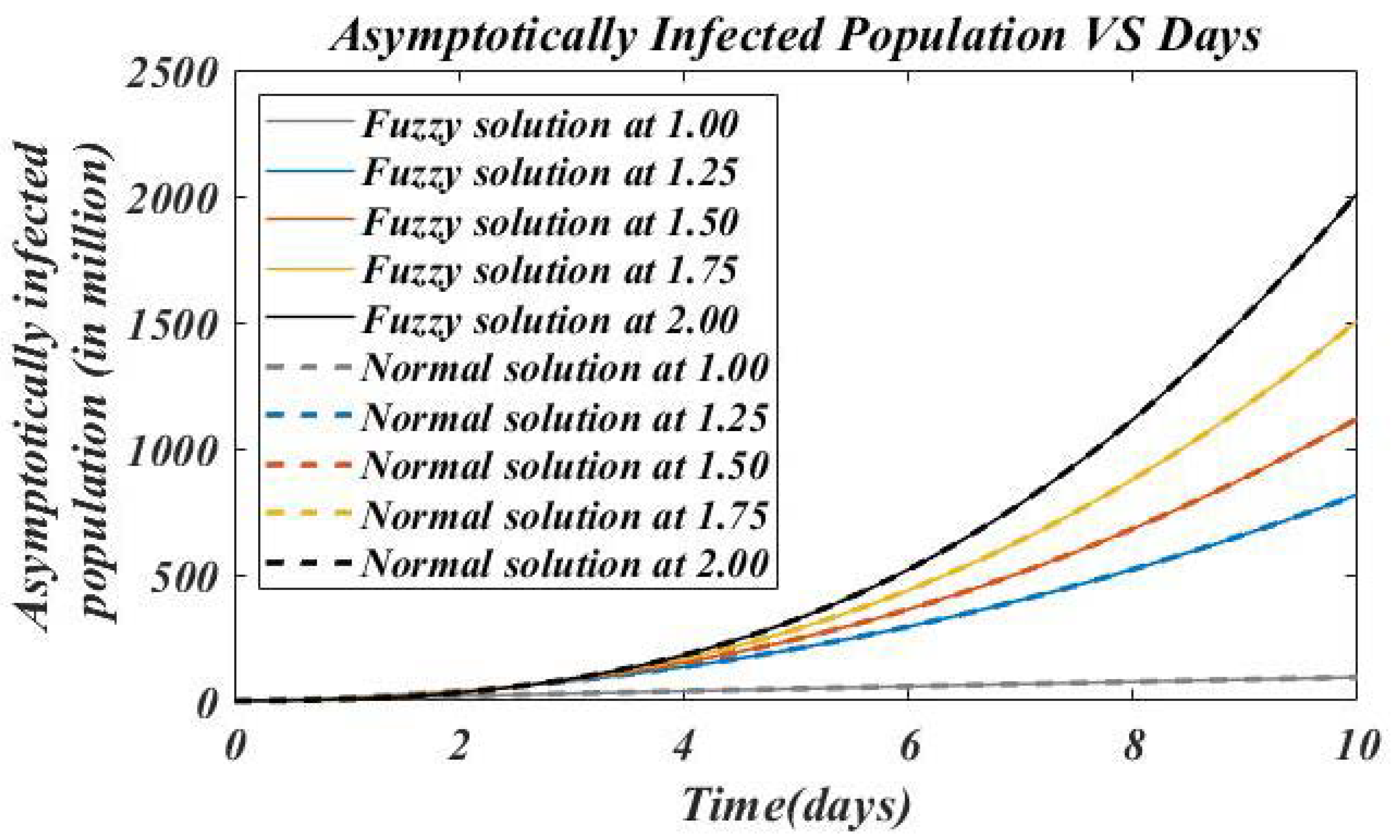
Here, we present the computational results based on the numerical scheme discussed above. Figure 1, Figure 2, Figure 3, Figure 4, Figure 5 and Figure 6 show a comparison of approximate fuzzy and approximate normal solutions for the considered model at various fractional orders for the given uncertainty. Figure 1 presents the susceptible population versus days; in Figure 2, the exposed population versus days; in Figure 3 the infected population versus days; in Figure 4, the recovered population versus days; in Figure 5, the asymptotically infected population versus days; and in Figure 6, the reservoir population versus days for a fuzzy and normal solution at 1.25, 1.50 and 1.75. Figure 7 shows the recovered population versus days and in Figure 8, the asymptotically infected population versus days for a fuzzy and normal solution at 1.00, 1.25, 1.50, 1.75 and 2.00. As the susceptible class value decreases, the exposed population grows, and the infection spreads at a different rate due to changing fractional orders. Similarly, when the number of death cases rises, the recovered class expands, the asymptotically infected class expands, and the virus population in the reservoir expands. We can see from the pictures that fuzziness, in combination with fractional order , provides global dynamics to nonlinear problems where the data are uncertain.
Remark 1.
According to the results, the lower bounded is a growing set-valued function, while the upper bounded is a decreasing one, indicating that the solutions are fuzzy numbers. It is also worth noting that under fuzzy differentiability, identical findings can be derived in general circumstances.
Remark 2.
Given that stochastic and random parameters are more difficult to address, and that uncertainty might contribute to an increase in computation costs, using fuzzy notions to model such real-world systems may be the best option.
5. Conclusions
In this paper, we present an analytical investigation of the fractional order COVID-19 model (3) for existence–uniqueness results, as well as numerical simulations. We used the Schauder’s fixed point theorem to prove that the solution to the fuzzy fractional-order model of COVID-19 exists and is unique. Using the fuzzy Laplace transform and the Adomian decomposition approach, we established a reasonable strategy for obtaining an approximate solution for the recommended model. We compared fuzzy and normal results for up to three phrases to demonstrate the utility of this method. We discovered that fuzziness combined with a fractional calculus technique yielded outstanding global dynamics in instances where data uncertainty exists. For future research, we recommend that readers revisit the problem for stochastic differential operators, optimal control and sensitivity analysis. Furthermore, the provided results can be compared to simulations for different fractional derivatives.
Author Contributions
Formal analysis, A.U.K.N.; Project administration, M.B.J.; Supervision, A.S.A. and A.U.K.N.; Writing–original draft, R.S.; Writing–review & editing, M.B.J. All authors have read and agreed to the published version of the manuscript.
Funding
This research was funded by [Imam Mohammad Ibn Saud Islamic University] grant number [21-13-18-069] and the APC was funded by [Imam Mohammad Ibn Saud Islamic University].
Institutional Review Board Statement
Not applicable.
Informed Consent Statement
Not applicable.
Data Availability Statement
No new data were created this study.
Acknowledgments
The authors extend their appreciation to the Deanship of Scientific Research at Imam Mohammad Ibn Saud Islamic University for funding this work through Research Group no. 21-13-18-069.
Conflicts of Interest
The authors declare that they have no known competing financial interest or personal relationships that could have appeared to influence the work reported in this paper.
References
- Chan, J.F.W.; Kok, K.H.; Zhu, Z.; Chu, H.; To, K.K.W.; Yuan, S.; Yuen, K.Y. Genomic characterization of the 2019 novel human-pathogenic coronavirus isolated from a patient with atypical pneumonia after visiting Wuhan. Emerg. Microbes Infect. 2020, 9, 221–236. [Google Scholar] [CrossRef] [PubMed] [Green Version]
- Lu, H.; Stratton, C.W.; Tang, Y.W. Outbreak of pneumonia of unknown etiology in Wuhan, China: The mystery and the miracle. J. Med. Virol. 2020, 92, 401. [Google Scholar] [CrossRef] [PubMed] [Green Version]
- Ji, W.; Wang, W.; Zhao, X.; Zai, J.; Li, X. Homologous recombination within the spike glycoprotein of the newly identified coronavirus may boost cross-species transmission from snake to human. J. Med. Virol. 2020, 92, 433–440. [Google Scholar] [CrossRef]
- Fahmi, I. World Health Organization Coronavirus Disease 2019 (COVID-19) Situation Report; WHO: Geneva, Switzerland, 2019. [Google Scholar]
- Chen, Y.; Guo, D. Molecular mechanisms of coronavirus RNA capping and methylation. Virol. Sin. 2016, 31, 3–11. [Google Scholar] [CrossRef] [PubMed] [Green Version]
- Wang, L.F.; Shi, Z.; Zhang, S.; Field, H.; Daszak, P.; Eaton, B.T. Review of bats and SARS. Emerg. Infect. Dis. 2006, 12, 1834. [Google Scholar] [CrossRef]
- Ge, X.Y.; Li, J.L.; Yang, X.L.; Chmura, A.A.; Zhu, G.; Epstein, J.H.; Mazet, J.K.; Hu, B.; Zhang, W.; Peng, C.; et al. Isolation and characterization of a bat SARS-like coronavirus that uses the ACE2 receptor. Nature 2013, 503, 535–538. [Google Scholar] [CrossRef]
- Lu, R.; Zhao, X.; Li, J.; Niu, P.; Yang, B.; Wu, H.; Wang, W.; Song, H.; Huang, B.; Zhu, N.; et al. Genomic characterisation and epidemiology of 2019 novel coronavirus: Implications for virus origins and receptor binding. Lancet 2020, 395, 565–574. [Google Scholar] [CrossRef] [Green Version]
- Zhou, P.; Yang, X.L.; Wang, X.G.; Hu, B.; Zhang, L.; Zhang, W.; Si, H.-R.; Zhu, Y.; Li, B.; Huang, C.-L.; et al. A pneumonia outbreak associated with a new coronavirus of probable bat origin. Nature 2020, 579, 270–273. [Google Scholar] [CrossRef] [Green Version]
- Tian, X.; Li, C.; Huang, A.; Xia, S.; Lu, S.; Shi, Z.; Lu, L.; Jiang, S.; Yang, Z.; Wu, Y.; et al. Potent binding of 2019 novel coronavirus spike protein by a SARS coronavirus-specific human monoclonal antibody. Emerg. Microbes Infect. 2020, 9, 382–385. [Google Scholar] [CrossRef] [Green Version]
- Ahmed, S.F.; Quadeer, A.A.; McKay, M.R. Preliminary identification of potential vaccine targets for 2019-nCoV based on SARS-CoV immunological studies. Viruses 2020, 12, 254. [Google Scholar] [CrossRef] [Green Version]
- Chaudhury, S.; Berrondo, M.; Weitzner, B.D.; Muthu, P.; Bergman, H.; Gray, J.J. Benchmarking and analysis of protein docking performance in Rosetta v3. 2. PLoS ONE 2011, 6, e22477. [Google Scholar] [CrossRef] [PubMed] [Green Version]
- Khan, M.A.; Atangana, A. Modeling the dynamics of novel coronavirus (2019-nCov) with fractional derivative. Alex. Eng. J. 2020, 59, 2379–2389. [Google Scholar] [CrossRef]
- Agarwal, R.P.; Lakshmikantham, V.; Nieto, J.J. On the concept of solution for fractional differential equations with uncertainty. Nonlinear Anal. Theory Methods Appl. 2010, 72, 2859–2862. [Google Scholar] [CrossRef]
- Asjad, M.I.; Aleem, M.; Ahmadian, A.; Salahshour, S.; Ferrara, M. New trends of fractional modeling and heat and mass transfer investigation of (SWCNTs and MWCNTs)-CMC based nanofluids flow over inclined plate with generalized boundary conditions. Chin. J. Phys. 2020, 66, 497–516. [Google Scholar] [CrossRef]
- Abbas, A.; Shafqat, R.; Jeelani, M.B.; Alharthi, N.H. Significance of Chemical Reaction and Lorentz Force on Third-Grade Fluid Flow and Heat Transfer with Darcy-Forchheimer Law over an Inclined Exponentially Stretching Sheet Embedded in a Porous Medium. Symmetry 2022, 14, 779. [Google Scholar] [CrossRef]
- Abbas, A.; Shafqat, R.; Jeelani, M.B.; Alharthi, N.H. Convective Heat and Mass Transfer in Third-Grade Fluid with Darcy–Forchheimer Relation in the Presence of Thermal-Diffusion and Diffusion-Thermo Effects over an Exponentially Inclined Stretching Sheet Surrounded by a Porous Medium: A CFD Study. Processes 2022, 10, 776. [Google Scholar] [CrossRef]
- Kaleva, O. Fuzzy differential equations. Fuzzy Sets Syst. 1987, 24, 301–317. [Google Scholar] [CrossRef]
- Lupulescu, V. Fractional calculus for interval-valued functions. Fuzzy Sets Syst. 2015, 265, 63–85. [Google Scholar] [CrossRef]
- Arshad, S.; Lupulescu, V. Fractional differential equation with the fuzzy initial condition. Electron. J. Differ. Equ. 2011, 34, 1–8. [Google Scholar]
- Benchohra, M.; Cabada, A.; Seba, D. An existence result for nonlinear fractional differential equations on Banach spaces. Bound. Value Probl. 2009, 2009, 628916. [Google Scholar] [CrossRef] [Green Version]
- Belmekki, M.; Nieto, J.; Rodriguez-Lopez, R. Existence of periodic solution for a nonlinear fractional differential equation. Bound. Value Probl. 2009, 2009, 324561. [Google Scholar] [CrossRef] [Green Version]
- Park, J.Y.; Han, H.K. Existence and uniqueness theorem for a solution of fuzzy Volterra integral equations. Fuzzy Sets Syst. 1999, 105, 481–488. [Google Scholar] [CrossRef]
- Ali, N.; Khan, R.A. Existence of positive solution to a class of fractional differential equations with three point boundary conditions. Math. Sci. Lett. 2016, 5, 291–296. [Google Scholar] [CrossRef]
- Khan, R.A.; Shah, K. Existence and uniqueness of solutions to fractional order multi-point boundary value problems. Commun. Appl. Anal. 2015, 19, 515–525. [Google Scholar]
- Lakshmikantham, V.; Leela, S. Nagumo-type uniqueness result for fractional differential equations. Nonlinear Anal. 2009, 71, 2886–2889. [Google Scholar] [CrossRef]
- Miller, K.S.; Ross, B. An Introduction to the Fractional Calculus and Fractional Differential Equations; Wiley: Hoboken, NJ, USA, 1993. [Google Scholar]
- Lakshmikantham, V.; Vatsala, A.S. Basic theory of fractional differential equations. Nonlinear Anal. Theory Methods Appl. 2008, 69, 2677–2682. [Google Scholar] [CrossRef]
- Perfilieva, I. Fuzzy transforms: Theory and applications. Fuzzy Sets Syst. 2006, 157, 993–1023. [Google Scholar] [CrossRef]
- Salahshour, S.; Allahviranloo, T. Application of fuzzy differential transform method for solving fuzzy Volterra integral equations. Appl. Math. Model. 2013, 37, 1016–1027. [Google Scholar] [CrossRef]
- Allahviranloo, T.; Salahshour, S.; Abbasbandy, S. Explicit solutions of fractional differential equations with uncertainty. Soft Comput. 2012, 16, 297–302. [Google Scholar] [CrossRef]
- Allahviranloo, T.; Ahmadi, M.B. Fuzzy laplace transforms. Soft Comput. 2010, 14, 235. [Google Scholar] [CrossRef]
- Zhu, Y. Stability analysis of fuzzy linear differential equations. Fuzzy Optim. Decis. Mak. 2010, 9, 169–186. [Google Scholar] [CrossRef]
- Niazi, A.U.K.; He, J.; Shafqat, R.; Ahmed, B. Existence, Uniqueness, and Eq–Ulam-Type Stability of Fuzzy Fractional Differential Equation. Fractal Fract. 2021, 5, 66. [Google Scholar] [CrossRef]
- Iqbal, N.; Niazi, A.U.K.; Shafqat, R.; Zaland, S. Existence and Uniqueness of Mild Solution for Fractional-Order Controlled Fuzzy Evolution Equation. J. Funct. Spaces 2021, 2021, 5795065. [Google Scholar] [CrossRef]
- Shafqat, R.; Niazi, A.U.K.; Jeelani, M.B.; Alharthi, N.H. Existence and Uniqueness of Mild Solution Where α∈(1,2) for Fuzzy Fractional Evolution Equations with Uncertainty. Fractal Fract. 2022, 6, 65. [Google Scholar] [CrossRef]
- Abuasbeh, K.; Shafqat, R.; Niazi, A.U.K.; Awadalla, M. Local and Global Existence and Uniqueness of Solution for Time-Fractional Fuzzy Navier–Stokes Equations. Fractal Fract. 2022, 6, 330. [Google Scholar] [CrossRef]
- Ahmad, S.; Ullah, A.; Shah, K.; Salahshour, S.; Ahmadian, A.; Ciano, T. Fuzzy fractional-order model of the novel coronavirus. Adv. Differ. Equations 2020, 2020, 472. [Google Scholar] [CrossRef]
- Gottwald, S. Fuzzy Set Theory and Its Applications; Kluwer Academic Publishers: Dordrecht, The Netherlands, 1991; ISBN 0-7923-9075-X. [Google Scholar]
- Zadeh, L.A. Fuzzy sets. In Fuzzy Sets, Fuzzy Logic, and Fuzzy Systems; World Scientific: Singapore, 1996; pp. 394–432. [Google Scholar]
Figure 1.
Illustration of approximate fuzzy and normal susceptible compartment solutions for three terms at given uncertainty levels versus fractional order.
Figure 1.
Illustration of approximate fuzzy and normal susceptible compartment solutions for three terms at given uncertainty levels versus fractional order.

Figure 2.
Illustration of approximate fuzzy and normal exposed compartment solutions for three terms at given uncertainty levels versus fractional order.
Figure 2.
Illustration of approximate fuzzy and normal exposed compartment solutions for three terms at given uncertainty levels versus fractional order.

Figure 3.
Illustration of approximate fuzzy and normal infected compartment solutions for three terms at given uncertainty levels versus fractional order.
Figure 3.
Illustration of approximate fuzzy and normal infected compartment solutions for three terms at given uncertainty levels versus fractional order.

Figure 4.
Illustration of approximate fuzzy and normal recovered compartment solutions for three terms at given uncertainty levels versus fractional order.
Figure 4.
Illustration of approximate fuzzy and normal recovered compartment solutions for three terms at given uncertainty levels versus fractional order.

Figure 5.
Illustration of approximate fuzzy and normal asymptotically infected compartment solutions for three terms at given uncertainty levels versus fractional order.
Figure 5.
Illustration of approximate fuzzy and normal asymptotically infected compartment solutions for three terms at given uncertainty levels versus fractional order.

Figure 6.
Illustration of approximate fuzzy and normal reservoir compartment solutions for three terms at given uncertainty levels versus fractional order.
Figure 6.
Illustration of approximate fuzzy and normal reservoir compartment solutions for three terms at given uncertainty levels versus fractional order.

Figure 7.
Illustration of approximate fuzzy and normal recovered compartment solutions for five terms at given uncertainty levels versus fractional order.
Figure 7.
Illustration of approximate fuzzy and normal recovered compartment solutions for five terms at given uncertainty levels versus fractional order.

Figure 8.
Illustration of approximate fuzzy and normal asymptotically infected compartment solutions for five terms at given uncertainty levels versus fractional order.
Figure 8.
Illustration of approximate fuzzy and normal asymptotically infected compartment solutions for five terms at given uncertainty levels versus fractional order.


Table 1.
Description of the model’s parameters (3).
Table 1.
Description of the model’s parameters (3).
| Notation | Parameters Description | Numerical Value |
|---|---|---|
| Birth rate | 1 | |
| Death rate of infected population | ||
| Transmission coefficient | 0.05 | |
| Disease transmission coefficient | 0.001231 | |
| Signified incubation period | 0.001234, 0.05 | |
| Recovery rate of | 0.1389 | |
| Influence of virus from and to | 0.0398, 0.01 | |
| Amount of asymptotic infection | 0.1243 | |
| Transmissibility multiple | 0.02 | |
| Elimination rate of virus from | 0.01 | |
| Initial value of susceptible | 220 million | |
| Initial value of infected | 0.015 million | |
| Initial value of exposed | 100 million | |
| Initial value of asymptotically infected | 0.60 million | |
| Initial value of recovered | 0 million | |
| Initial value of reservoir | 0.1 million |
Publisher’s Note: MDPI stays neutral with regard to jurisdictional claims in published maps and institutional affiliations. |
© 2022 by the authors. Licensee MDPI, Basel, Switzerland. This article is an open access article distributed under the terms and conditions of the Creative Commons Attribution (CC BY) license (https://creativecommons.org/licenses/by/4.0/).
Share and Cite
MDPI and ACS Style
Alnahdi, A.S.; Shafqat, R.; Niazi, A.U.K.; Jeelani, M.B. Pattern Formation Induced by Fuzzy Fractional-Order Model of COVID-19. Axioms 2022, 11, 313. https://doi.org/10.3390/axioms11070313
AMA Style
Alnahdi AS, Shafqat R, Niazi AUK, Jeelani MB. Pattern Formation Induced by Fuzzy Fractional-Order Model of COVID-19. Axioms. 2022; 11(7):313. https://doi.org/10.3390/axioms11070313
Chicago/Turabian StyleAlnahdi, Abeer S., Ramsha Shafqat, Azmat Ullah Khan Niazi, and Mdi Begum Jeelani. 2022. "Pattern Formation Induced by Fuzzy Fractional-Order Model of COVID-19" Axioms 11, no. 7: 313. https://doi.org/10.3390/axioms11070313
Note that from the first issue of 2016, this journal uses article numbers instead of page numbers. See further details here.