
Assessing the Predictive Power of Online Social Media to Analyze COVID-19 Outbreaks in the 50 U.S. States


1
MIT Center for Collective Intelligence, Cambridge, MA 02140, USA
2
School of Electronics and Information Technology, Sun Yat-sen University, Guangzhou 510006, China
*
Author to whom correspondence should be addressed.
Future Internet 2021, 13(7), 184; https://doi.org/10.3390/fi13070184
Submission received: 2 June 2021
/
Revised: 9 July 2021
/
Accepted: 14 July 2021
/
Published: 20 July 2021
(This article belongs to the Section Big Data and Augmented Intelligence)
Abstract
:As the coronavirus disease 2019 (COVID-19) continues to rage worldwide, the United States has become the most affected country, with more than 34.1 million total confirmed cases up to 1 June 2021. In this work, we investigate correlations between online social media and Internet search for the COVID-19 pandemic among 50 U.S. states. By collecting the state-level daily trends through both Twitter and Google Trends, we observe a high but state-different lag correlation with the number of daily confirmed cases. We further find that the accuracy measured by the correlation coefficient is positively correlated to a state’s demographic, air traffic volume and GDP development. Most importantly, we show that a state’s early infection rate is negatively correlated with the lag to the previous peak in Internet searches and tweeting about COVID-19, indicating that earlier collective awareness on Twitter/Google correlates with a lower infection rate. Lastly, we demonstrate that correlations between online social media and search trends are sensitive to time, mainly due to the attention shifting of the public.
1. Introduction
“At every crucial moment, American officials were weeks or months behind the reality of the outbreak. Those delays likely cost tens of thousands of lives”. NYT 26 June 2020 [1].
Since the beginning of January 2020, the world has been turned upside down. Nothing is like it was before since the novel coronavirus disease was first reported in Wuhan, China, in December 2019 [2]. After initial blunders, China took energetic measures to combat the virus (e.g., the Wuhan shutdown) [3] while the Western world was still mostly complacent. Although epidemiologists had already warned at the end of January that COVID-19 would probably turn into a global crisis [4], politicians and the population in the U.S. and Western Europe alike initially ignored the problem. The virus was seen as something far away, that similar to SARS and the avian flu, would be active mostly in the high-density populations of Asia and then go away. Even when Italy was shaken with a virulent COVID-19 outbreak in February [5], which closed down the northern industrial heartland of Veneto, the U.S. authorities were still mostly ignoring the problem [6]. Only when in mid-March, New York started seeing soaring infection rates did the population and the politicians start taking the disease seriously. This behavior is perfectly reflected in the Google search trend and the Twitter activity, motivating our research question: Is a state or political entity better capable of dealing with an infectious disease if the collective awareness is raised early on in the course of the disease? Does a population actively searching for information about COVID-19 and showing a robust dialog on Twitter about this topic deal more efficiently with the disease?
In the earlier related research, it has been illustrated that data from online social media and Internet searches are correlated with several epidemics that have previously happened, such as seasonal influenza epidemics [7], Dengue [8], MERS [9] and H1N1 [10]. Regarding COVID-19, several works [11,12,13,14] have demonstrated a significant correlation between the Internet search and the pandemic spreading among different countries. For instance, a Google Trends comparison with the number of infections in various countries was presented in [11], where it was found that initially the correlation between searches and infection rates in these countries was high with a lag of 0 to 12 days but decreased while the infection rate was still going up once the initial public interest in COVID-19 was tampering off. In [12], the authors compared the social media posts and search trends in China with the infection rate, albeit only until 11 February 2020. Although a correlation was found, its representativity is limited, as the period of the analysis was very short and restricted to China. Study [13] finds for 21 countries, the more citizens of a country search for “hand washing,” the lower is the infection rate. However, this is also a very short study, only covering the period from 19 January to 18 February 2020, and thus of restricted generalizability. In [14], it was found that searching for “loss of smell” from 1 December 2019 to 25 March 2020 in Italy, Spain, UK, U.S., Germany, France, Iran and the Netherlands directly correlated with the infection rate in these countries. While these studies demonstrate the initial predictive power of search trends and social media posting for predicting the infection rate, they are all restricted by the relatively short observation period during the onset of the pandemic, as well as the limited comparability of the observed geographies. Therefore, it still remains unclear what regional factors the Internet’s predictive abilities may relate to and whether they are useful at surveilling the spread of the disease. Our hypothesis is that there will be a statistically significant correlation in the Google search and tweeting behavior of a U.S. polity such as a state or a city and its COVID-19 infection rate, which thus will give valuable input to policymakers, governments, and healthcare providers to better prepare and deal with potential future waves of the COVID-19 and other epidemics.
In this work, using the data from 50 states of the United States, we conduct a comparative study about the role of online social media and search trends in the COVID-19 epidemic. We show that the daily number of COVID-19 related tweets on Twitter exhibits a strong but state-different lag correlation with newly confirmed cases. The same can be observed on the Google Trends index using coronavirus-related search terms. These state-differences in correlation strength and lag are closely related to a state’s demographics, quantitively measured by a state’s population size and density, air traffic volume and economic development. Further, our analysis on the state-level early COVID-19 incidents demonstrates a significantly negative correlation between the lag and the early infection rate, implying that an actively engaged population that searches for information and tweets about COVID-19 more ahead of the outbreak correlates with a lower infection rate. Lastly, based on extended data, we find that the size of the correlation between online social media and search trends and COVID-19 rates varies across time. While explaining the reduced correlation of our initial metric for later data collected in the summer and fall of 2020, we identify a new metric that correlates with the fall 2020 COVID-19 testing trend.
The remainder of the paper is organized as follows: first, we explain the method and process we applied for data analysis. We then present our results for the first four months of the pandemic, where tweets and Google search trends showed a high correlation with the infection rate. We subsequently investigate the second period of the pandemic starting in June 2020 until October 2020, where we find that COVID testing correlates with Twitter and Google search behavior, applying the same method. We finish the paper with conclusions.
2. Materials and Methods
COVID-19 Twitter Data. The COVID-19 tweets on Twitter are acquired from an open COVID-19 Twitter chatter dataset [15], which is a collection of the identifiers of tweets specifically using coronavirus-related keywords (coronavirus, 2019nCoV, COVD19, CoronavirusPandemic, CoronaOutbreak, etc.), starting from 27 January 2020. After hydrating the full JSON objects from these tweets’ identifiers, we extract the daily number of tweets in the U.S. at the state level according to a tweet’s location. This means that according to the Twitter developer API description, we lose 98% of the tweets, but we can be certain that they indeed come from a specific location. Specifically, we first identify all geo-located tweets (i.e., tweets associated with a geographic place), only retaining tweets with a location in the U.S. Then, we assign a tweet to a state using its specific location, such as city and town (see the heatmap of the number of geo-located tweets in 50 U.S. states until 30 September 2020 in the SI Figure S2). The study period and the smooth operation of the Twitter data are the same as that of COVID-19 infection cases. We would like to emphasize that the Twitter data used in this work are the raw count of tweets, i.e., the daily number of COVID-19 tweets in each state. In particular, the correlation quantities (i.e., and defined in this work) for each state can be obtained by looking at the curve pattern of COVID-19-related tweets. Therefore, as we iteratively correlate two curves, both representative of the size of a state, to obtain the best possible correlation value, there is no need to normalize it with the total number of tweets sent in a state.
Google Trends and Keywords. As the most used search engine in the U.S., Google Trends (https://www.google.com/trends, accessed on 1 October 2020) provides an excellent proxy for Internet-search trends. The Google Trends index measures the search activity of a term compared to the most actively searched keyword for a selected region. For each individual state, we use a combination of a COVID-related keyword and the state’s full name as an integrated search term throughout this paper. We also tried to use Google Trends at the state level; however, this led to very similar curves across all states. Specifically, for studying the U.S.’ interest in the pandemic, we use the pytrends API to track three respective keywords, ‘coronavirus’, ‘COVID’ and ‘COVID-19′ on Google Trends among 50 U.S. states. For studying COVID testing, we select the corresponding keyword ‘COVID testing’ for querying Google Trends. After downloading the data, we smooth them with the same parameter used in the real data (i.e., 3 days-average for the three general keywords, 7 days average for ‘COVID testing’). The time parameter is set to two weeks before the COVID-19 data in each state to fully capture the baseline interest.
U.S. Interest in Google Trends. We did a cross-sectional comparison of several search interests within the U.S. region. Particularly, we downloaded the Google Trends index of ‘coronavirus’, ‘sports’, ‘music’, ’news’ and ‘weather’ from 15 January 2020 to September 30, 2020, by setting the search area to the U.S. As a purely intuitive comparison, we did not apply a smoothing operation to the data.
COVID-19 Testing Trends in U.S. We obtain the state-by-state testing trend through the COVID Tracking Project (https://coronavirus.jhu.edu/testing/individual-states, access on 1 October 2020), which is as far as we know the best source to cite for daily U.S. test numbers. We include the data from 1 February 2020 to 30 September 2020 in this study. To reduce the effect of noise and to get better insights from the trends, we smooth the data with a 7-day-average, similarly to Johns Hopkins, which use the same data source for its COVID-19 Testing Insights Initiative (https://coronavirus.jhu.edu/testing/individual-states, access on 1 October 2020).
COVID-19 Infection Cases in U.S. The COVID-19 confirmed cases are collected from the New York Times (https://www.nytimes.com/, accessed on 1 October 2020) based on reports from state and local health agencies. We exclude Puerto Rico and the District of Columbia since some Internet data for these two regions are unavailable. As a result, 50 U.S. states’ daily number of cases are used in this study. We start searching data from 20 January 2020, which is the date when the first U.S. case was reported. The specific study period of each state is from the date of the first confirmed case in this state to 30 May 2020 and is then extended to 30 September 2020 for studying the variation of correlation strength. We smooth the raw data by a 3-days-average to reduce the noise.
Correlation analysis. The Spearman correlation is employed in this study using Python’s SciPy function. Specifically, we conduct lagged correlation analyses to assess the temporal relationships between Internet data and the COVID-19 pandemic. For each state, we right-shift the daily Internet data from Twitter and Google Trends (with different search terms) by a variable lag and calculate the Spearman correlation to the daily reported COVID-19 cases. The maximum lag is set to 40 days. The Spearman correlation is also used to examine the correlation between the and the state’s variables, and between the and the early infection rate, at significance levels from * < 0.1 to *** < 0.01.
Proxy of air traffic flow. Using the Air Carrier Activity Information System database (https://www.faa.gov/airports/planning_capacity/passenger_allcargo_stats/passenger/collection/, accessed on 1 October 2020), we obtain the enplanement data at every commercial service airport in the U.S. for 2017 and 2018. As a proxy of a state’s air traffic flow, we calculate the sum of the enplanements of all airports located in a state.
3. Results
3.1. Lagged Correlations for Google Trend and Twitter
We first looked at COVID-19 infections, Twitter tweets and Google search data for all 50 U.S. states in early 2020 when the pandemic first appeared in the U.S. Specifically, we gathered state-level daily COVID-19 confirmed cases from 20 January 2020 to 30 May 2020. For the same period, we quantified the number of COVID-19 related tweets in each individual state by analyzing the geographic information from an open COVID-19 Twitter chatter dataset [15] (see Methods for detail). For Google Trends, we searched the data within a state by using a combination of one of three keywords (‘coronavirus’, ’COVID’ and ‘COVID-19′) and the state’s full name as an integrated search input (e.g., ‘coronavirus Massachusetts’). To capture the baseline interest before the pandemic, we set the starting time two weeks earlier than the COVID-19 outbreak date in a given state. It is known that the novel coronavirus was identified as the cause of this disease in early January and was then officially named novel coronavirus pneumonia by the NHC of China and later ‘coronavirus disease 2019’ (usually abbreviated as COVID-19, COVID) by the WHO in February. Therefore, we believe the selected three keywords ‘coronavirus’, ‘COVID’ and ‘COVID-19’ are the most likely search terms for individuals and thus are sufficient to include most Internet content related to COVID-19 in our search period. We used the combination of keywords and states’ names because residents are usually more concerned about their local situation of the pandemic, and thus, such an integrated search term more reasonably reflects the local Internet interest for COVID-19. We find that without adding the state’s full name, the search trends with the above keywords would become too similar in all 50 states (see SI Figure S1), which is undesirable to investigate the differences in state-by-state interest.
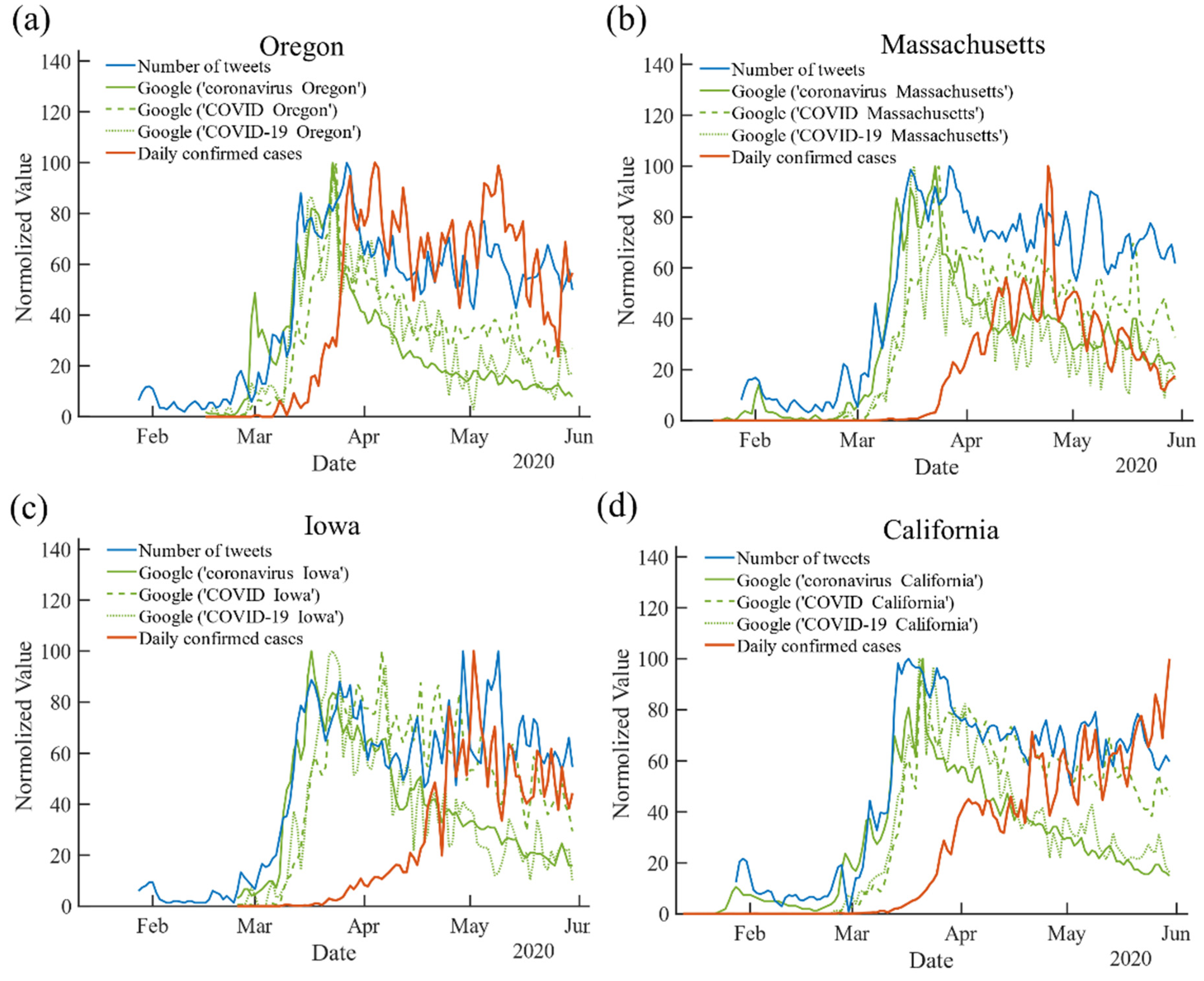
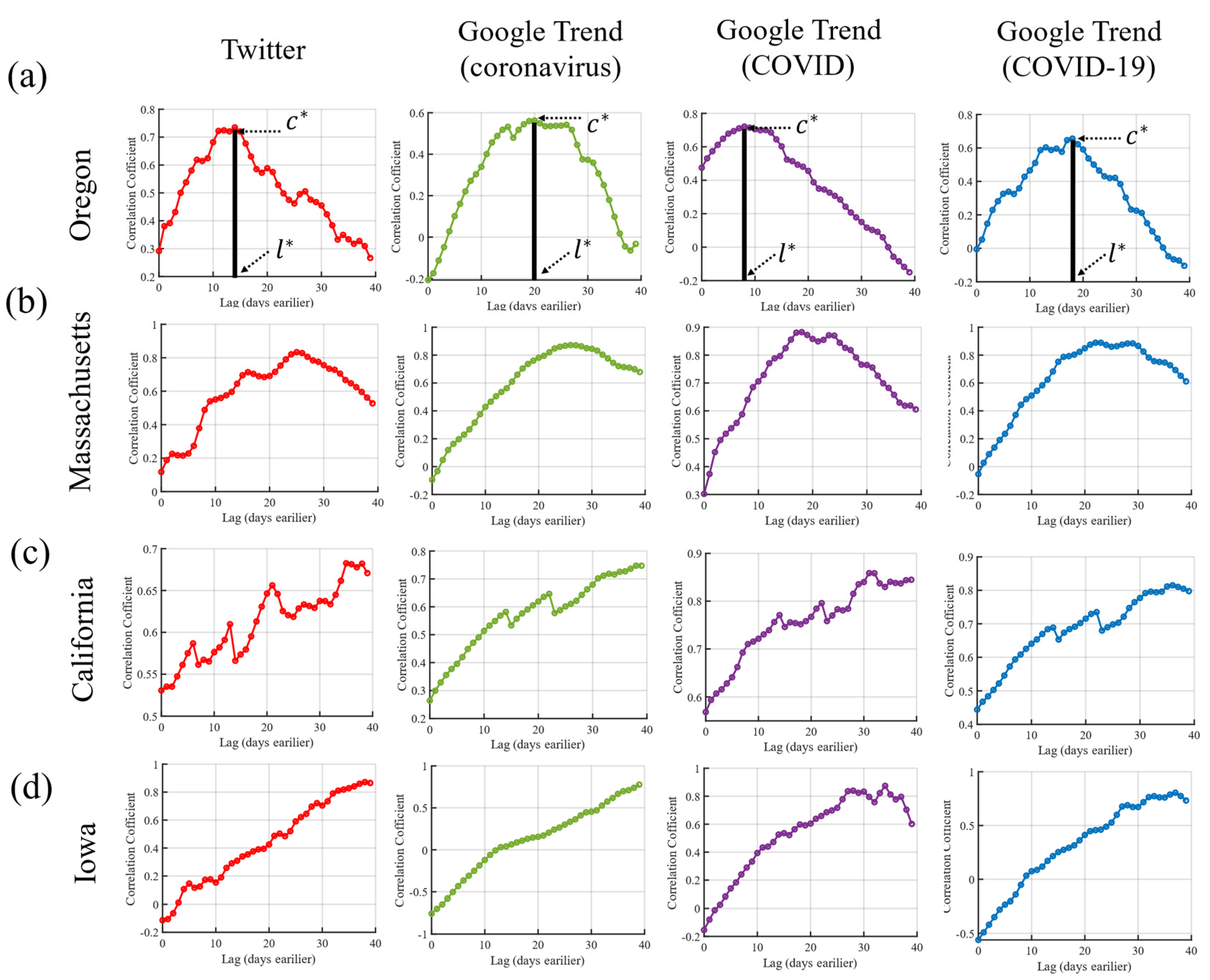
In Figure 1, we illustrate the comparison among the daily confirmed cases, the number of COVID-19 related tweets and the Google Trends indexes (with different search terms) in Oregon, Massachusetts, Iowa and California up to 30 May 2020 (see Methods for details of data processing). One can observe that the overall graph patterns are different between states. We then investigated the relationship between the COVID-19 pandemic spreading and the Internet data in all 50 U.S. states. Figure 2 shows the lagged Spearman correlation between the Internet data from Twitter and Google Trends and the reported COVID-19 cases for the selected four states. To quantify the correlation strength of the tweeting behavior and the search activity for an individual state, we denote as the highest correlation coefficient. In principle, a larger indicates a higher accuracy in correlating with the state-level pandemic. Besides, we define as the optimal lag achieving . In other words, when the curve of Internet data is right-shifted by days, it will most closely resemble the curve of COVID-19 daily infection. Therefore, itself is a direct metric to measure the distance between the two ’spikes’ of two curves, i.e., the time of the outbreak of the Internet’s collective awareness before the outbreak of epidemic. A larger corresponds to an earlier peak of Internet searches and tweeting about COVID-19, indicating that residents start being active on the Internet earlier. An additional advantage of using is that it can be automatically quantified through the lagged correlation analysis. In other words, it is parameter-free and is an intrinsic quantity expressed purely from the observed data. We find that and are quite different among different states and between Google Trends and Twitter (see Figure 2). For instance, for Massachusetts, is 0.80 with 27 using the Twitter data and is up to 0.90 with 17 for tracking ‘COVID Massachusetts’ on Google Trends. For California, the of Twitter and of ‘coronavirus California’ on Google Trends are 0.67 and 0.75, respectively, while the for both is above 30 days.
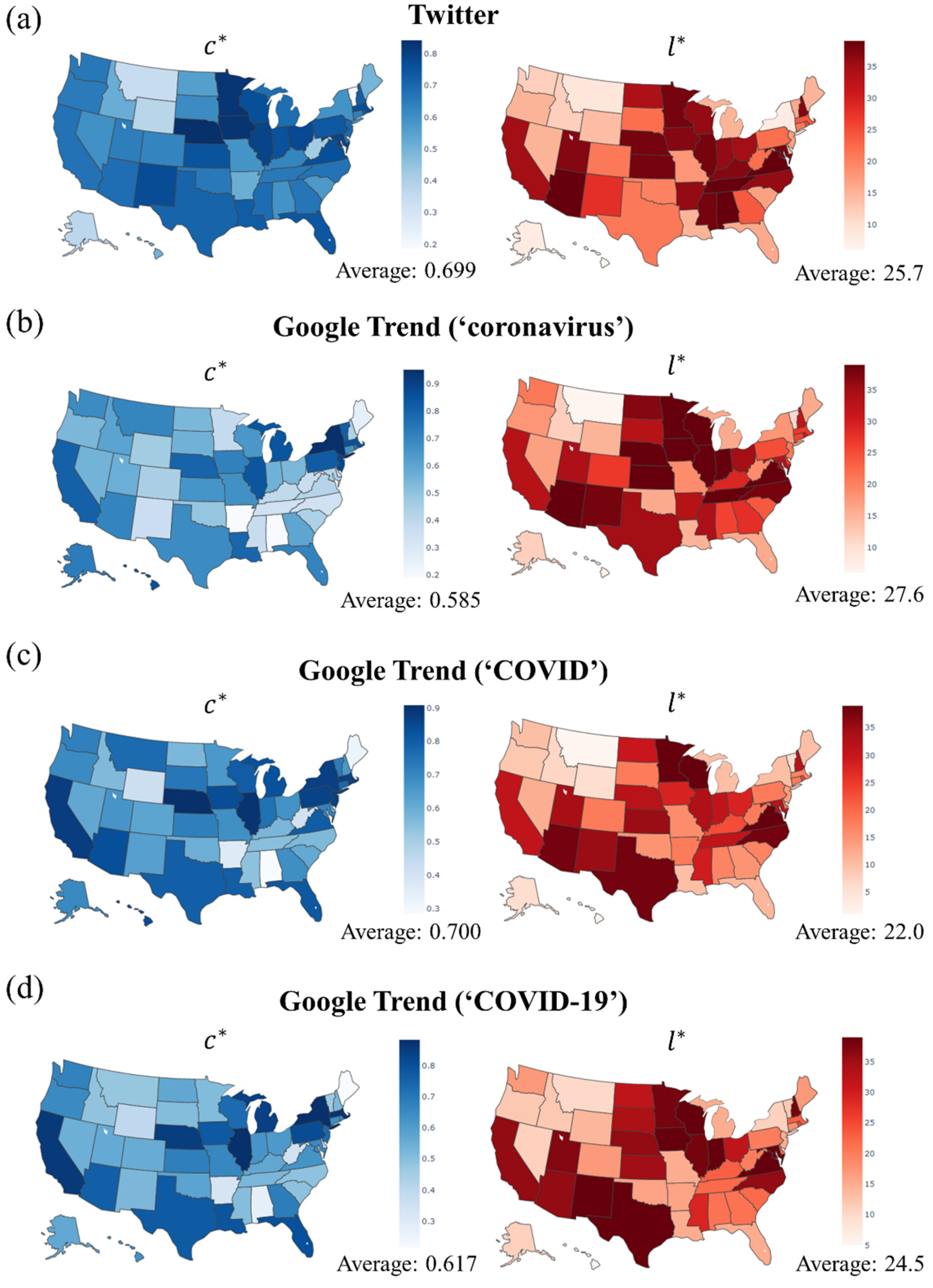
Figure 3 presents the distribution of and for Twitter and Google Trends for all 50 U.S. states. The average of from Twitter is 0.70, while is ranging from 0.59 to 0.70 for Google Trends using the search keyword ‘COVID.’ These results imply that the tweeting activity and search interest indeed are correlated with the COVID-19 spreading. On the other hand, the average on Twitter is about 26 days, revealing a smaller delay of the Twitter platform. Indeed, we find that and on Twitter are significantly correlated with < 0.001 (see the correlation coefficient between and in Supplementary Table S1), meaning that earlier collective tweeting may result in more accurate prediction. For Google Trends, the average of the keyword ‘coronavirus’ (27.6) is somewhat larger than for ‘COVID’ (22.0) and ‘COVID-19′ (25.0). An explanation could be that the majority of people searched for the word ‘coronavirus’ since the pandemic initially was reported under this name, while the names ’COVID’ and ‘COVID-19′ were formally proposed by the WHO at the end of February 2020.
3.2. Correlation between and State Conditions
We find that the wide difference of among the 50 states is partially related to a state’s economic and social conditions. Specifically, we consider population demographics, air traffic flow and the economic development level, which can be quantitively characterized by the following proxies. A state’s population size as of 2019 is estimated by the U.S. Census Bureau, along with the population density measured by the number of residents per square mile. The air traffic flow is measured by enplanement (i.e., the number of passengers boarding) in 2017 and 2018 (see details in the Methods Section). Besides, we collected each state’s gross domestic product (GDP) as well as the GDP per capita as of the 2019 4th quarter to measure economic output.
We calculated the Spearman correlation coefficient between these six variables and the of Twitter volume and Google Trends index, finding a significantly positive correlation, as shown in Table 1. In particular, the more people, the higher population density, the higher air traffic and wealth a state has, the higher the correlation of the Twitter and Google Trends with the COVID-19 pandemic is. This makes intuitive sense, as higher income is correlated with higher education, and higher geographic mobility leads to higher information exchange, both raising early awareness of the pandemic. There is no significant correlation between and the states’ demographic variables.
3.3. Correlation between Early Infected Rate and /
We further investigated the correlation between a population actively engaged on social media with the outbreak of the infection. Specifically, we focused on the early stage of the COVID-19 outbreak in the 50 U.S. states, a period when the government had not yet started to take serious control measures. The infection rate in this stage is a reasonable proxy to measure the extent to which a state’s residents rely on their individual awareness to protect themselves again the pandemic. Quantitively, we define the early infection rate as the proportion of residents being infected in the earliest days since the state-level first case was confirmed (see the distribution of the early infection rate among 50 states in SI Figure S3).
Having calculated both correlation strengths of Internet search and Twitter data and the early infection rate, we computed the relationship between the two. Surprisingly, we discovered a strong negative correlation between and the early infection rate, with varying from 1 week to 3 weeks, as shown in Table 2. This relationship indicates that the earlier people start tweeting and searching, the lower the infection rate. In other words, the earlier people tweeted about ‘COVID-19’ and searched for it on Google, the less people got infected when the virus breaks out. Moreover, we also find a significantly negative correlation between and the infection rate using the Twitter data and Google Trends for the terms ‘COVID’ and ‘COVID-19’ on selected ’s (see Table 2), implying that the more predictive pro-active Internet-search behavior is, the lower the initial infected rate. Our assumption is that while each individual does not know that there will be a big outbreak, the aggregation of all people searching on Google or tweeting about COVID-19 indicates that there will be an outbreak. Note that we do not make a claim about causality. It could just be that becoming aware of COVID-19 increases the likelihood of a person experiencing flu-like symptoms getting tested for COVID-19, which means that more cases are detected. As the Wallstreet Journal reported [16], more than 90 patients in central China were hospitalized with pneumonia or coronavirus-like symptoms in October and November 2019, indicating that COVID-19 might have spread before people became aware of it. Similarly, we are only claiming lagged correlation with detected COVID-19 cases and Twitter and Google search behavior. It could be that raising awareness will increase the likelihood of getting tested, thus driving up the incidence rate in the different states.
3.4. The Variation of Correlation Strength over Time
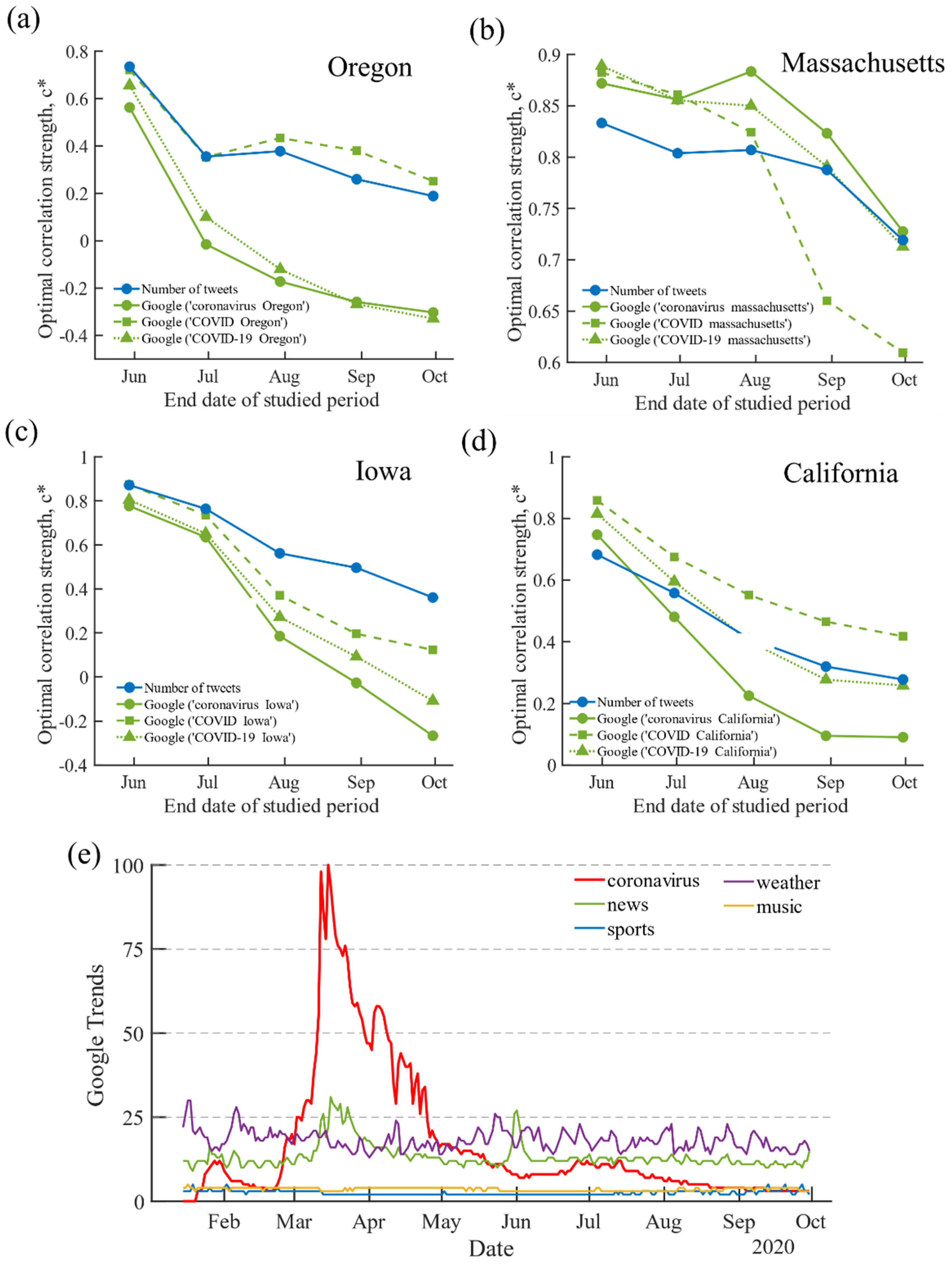
As the COVID-19 pandemic has been going on for many months, a lot has happened and changed. It is thus necessary to study the dynamic of the correlation between search and tweeting behavior and COVID-19 infections across time with extended data. Specifically, we further collected the state-level daily infection numbers, the COVID-keyword searches in Google Trends and the number of tweets in Twitter up until 30 September 2020. We find that the relationship between the COVID-19 pandemic spreading and the Internet data in all 50 U.S. states becomes weaker, especially in the last few months (see illustrations of four states in SI Figure S4). To further confirm the correlation variation over time, we calculate the optimal correlation strength (the highest lagged Spearman correlation) on the different studied periods for the above-mentioned four states, as shown in Figure 4a–d. We can clearly see that is almost always decreasing from spring to fall both for Google COVID-keyword searches and the number of tweets. Additionally, we carried out the same analysis for the remaining 46 states and found a similar reduction in , as shown in Supplementary Figure S5. In other words, the correlation of the COVID-keyword search and the number of tweets in the 50 U.S. states becomes weaker than at the beginning of the pandemic.
These results show that the COVID-19 related terms and tweets cease correlating highly as time passes, which confirms previous research analyzing time-sensitive public events. For instance, Google’s flu trends [17] or predicting U.S. elections ceased working well once people knew of its availability [18]. In the fall of 2020, COVID-19 had fully entered public awareness, and thus, people had no need to search for general information about this topic anymore. In other words, people were getting tired of terms such as ‘COVID’, and it just became part of daily life. As evidence, by collecting U.S. interest data on Google Trends (see Method for details), we found that the U.S. interest in searching ‘coronavirus’ peaked in the spring when the pandemic started to spread nationwide. After that, it was generally in line with daily search trends such as ‘music’ or ’sports’ (see Figure 4e).
3.5. Correlation Strength of ‘COVID Testing’ on Google
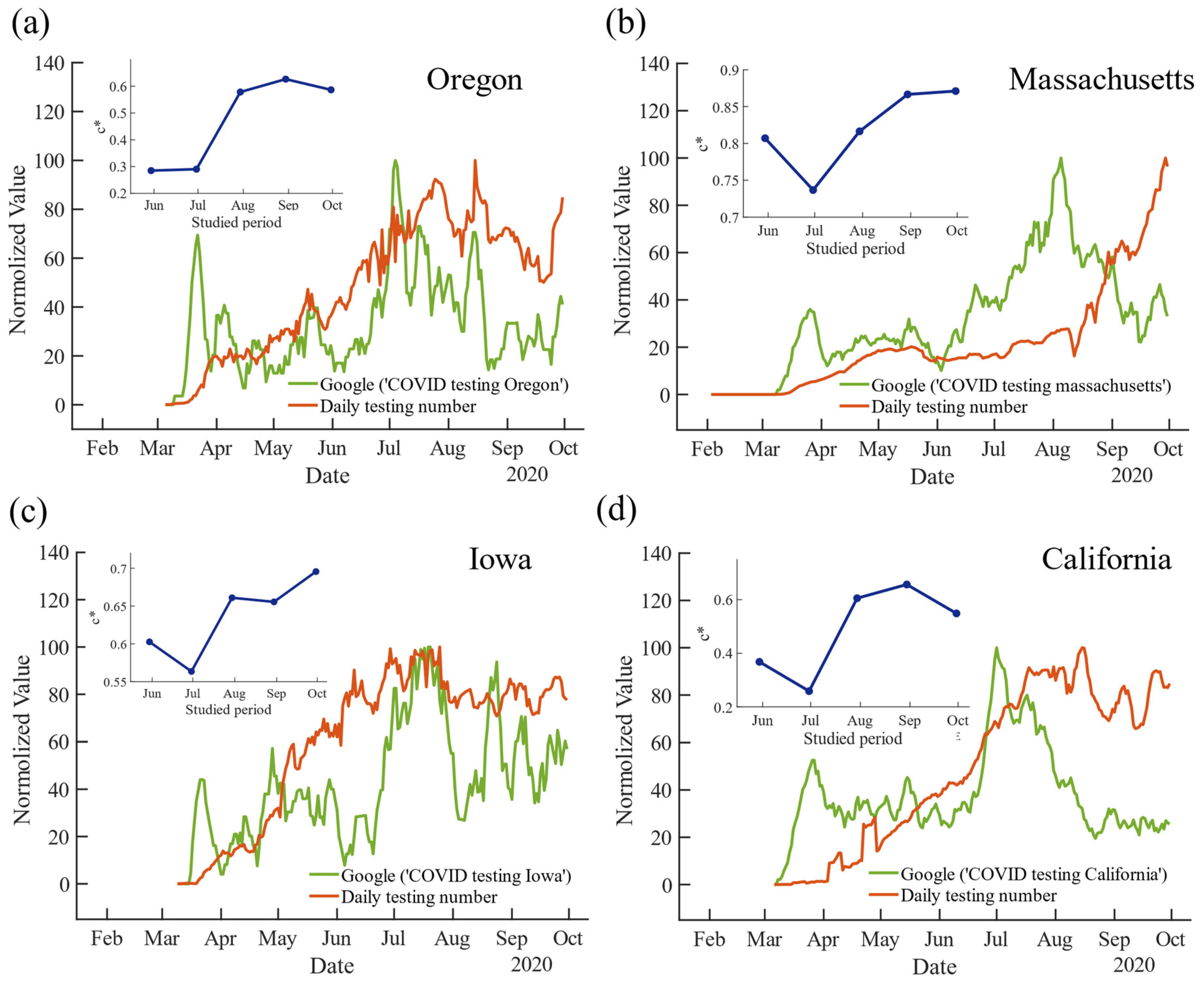
Finally, we demonstrate the correlation strength of other search terms that might capture people’s attention for the COVID-19-related situation within a state, finding that while it is still significant, the correlations are not as high as at the beginning of the COVID pandemic. One of the key concerns about COVID-19 is the testing that every state is doing to diagnose people with COVID-19 infection in order to gauge the spread of COVID-19 in the U.S. According to public data from the NYT [19], in the fall of 2020, the U.S. was conducting much more tests than in the summer or spring. To investigate the daily state-by-state testing trend through the Internet data, we carried out the following study: First, we obtained the state-by-state testing trend from 1 February 2020 to 30 September 2020, which is measured by the daily total tests in each individual state (see Methods for detail). Second, we queried Google Trends and downloaded the state-level data by using the search term ‘COVID testing’, Similarly, we combined the keyword with a state’s full name as an integrated search term and set the starting time two weeks before the first testing date. As there is a lot of noise in the raw data representing the testing trends in each state, we adopt a 7-days-average to smooth both the testing trend and the Google data to reduce the noise bias (see details in Methods). The comparison among the daily testing cases and the new Google Trends index in 4 different states is plotted in Figure 5, where one can clearly observe that the testing trend indeed exhibits lagged correlation with the online search trend, especially in the latest few months. Moreover, we studied the changes in the optimal correlation strength of ‘COVID testing’ as a function of the studied time period in four states (see Figure 5). Interestingly, we found that the achieved by the new index increases from spring to fall (a similar phenomenon is observed in the remaining 46 states, see SI Figure S6), which is in contrast to Figure 2, implying increasing correlation strength between the online search trend and the testing situation in the U.S.
4. Discussion and Conclusions
In conclusion, this study showed that there is a high but state-different correlation between the results of Google search and tweeting about COVID-19 related keywords and the number of confirmed COVID-19 cases among 50 U.S. states. These significant correlations occur as early as 27 days before confirmation of the infections, indicating the usefulness of Internet search and online social media tracking to surveil the pandemic’s outbreak locally. We further found that the differences in correlation strength between these states are closely related to a state’s demographics characterized by population size and density, air traffic and economic development. Most importantly, we discovered that if there is an actively tweeting population that leads a vibrant dialog on Twitter about COVID-19, the early detected infection rate will be lower. Similarly, the more ahead of the outbreak a population starts googling for COVID-19 information, the lower the early detected infection rate. It is quite likely that some sort of correlation between infection rate and Twitter activity about COVID-19 is to be expected. The contribution of this research is the insight that the size of the lag is negatively correlated with the infection rate, which illustrates that a population that expresses more concern about an upcoming crisis on social media will be better equipped to deal with the upcoming crisis. Note that we make no claims about causality between actual infection rate and size of the lag between actual COVID-19 outbreak and Twitter and Google search behavior. As mentioned above, it could just be that more COVID-19-aware states are testing more. It might well be that large numbers of asymptomatic infected people are missed in the infection count. Finding the actual infection rate at any given time would need continuous population-wide antibody testing, which has not been conducted. Besides, we wish to emphasize that developing full prediction models are not the focus of this work but to shed light on the collective behavior of the online social media the observed data describes. Lastly, we demonstrated that the correlation between online social media and a real-world event such as COVID-19 is sensitive to time, mainly due to the attention shifting of the public. As evidence, we provided an example with an interesting new metric correlated with the fall 2020 COVID-19 testing situation.
Supplementary Materials
The following are available online at https://www.mdpi.com/article/10.3390/fi13070184/s1, Figures S1–S6, Table S1.
Author Contributions
Conceptualization, P.A.G.; methodology, J.S. and P.A.G.; formal analysis, J.S.; writing—original draft preparation, J.S.; writing—review and editing, P.A.G.; All authors have read and agreed to the published version of the manuscript.
Funding
This research received no external funding.
Institutional Review Board Statement
Not applicable.
Informed Consent Statement
Not applicable.
Data Availability Statement
Source codes and all processed data used in this study is available at https://www.researchgate.net/profile/Jiachen_Sun2/publications accessed on 1 October 2020.
Conflicts of Interest
The authors declare no conflict of interest.
References
- Watkins, D.; Holder, J.; Glans, J.; Cai, W.; Carey, B.; White, J. How the virus won. New York Times. 24 June 2020. Available online: https://www.nytimes.com/interactive/2020/us/coronavirus-spread.html (accessed on 30 June 2020).
- Zhu, N.; Zhang, D.; Wang, W.; Li, X.; Yang, B.; Song, J.; Zhao, X.; Huang, B.; Shi, W.; Lu, R.; et al. A Novel Coronavirus from Patients with Pneumonia in China, 2019. N. Engl. J. Med. 2020, 382, 727–733. [Google Scholar] [CrossRef] [PubMed]
- Tian, H.; Liu, Y.; Li, Y.; Wu, C.-H.; Chen, B.; Kraemer, M.U.G.; Li, B.; Cai, J.; Xu, B.; Yang, Q.; et al. An investigation of transmission control measures during the first 50 days of the COVID-19 epidemic in China. Science 2020, 368, 638–642. [Google Scholar] [CrossRef] [PubMed] [Green Version]
- Li, R.; Pei, S.; Chen, B.; Song, Y.; Zhang, T.; Yang, W.; Shaman, J. Substantial undocumented infection facilitates the rapid dissemination of novel coronavirus (SARS-CoV-2). Science 2020, 368, 489–493. [Google Scholar] [CrossRef] [PubMed] [Green Version]
- Remuzzi, A.; Remuzzi, G. COVID-19 and Italy: What next? Lancet 2020, 395, 1225–1228. [Google Scholar] [CrossRef]
- Lipton, E.; Sanger, E.D.; Haberman, M.; Shear, D.M.; Mazzetti, M.; Branes, E.J. He Could Have Seen What Was Coming: Behind Trump’s Failure on the Virus. New York Times. 26 April 2020. Available online: https://www.nytimes.com/2020/04/11/us/politics/coronavirus-trump-response.html (accessed on 30 June 2020).
- Ginsberg, J.; Mohebbi, M.H.; Patel, R.S.; Brammer, L.; Smolinski, M.S.; Brilliant, L. Detecting influenza epidemics using search engine query data. Nature 2009, 457, 1012–1014. [Google Scholar] [CrossRef] [PubMed]
- Marques-Toledo, C.D.A.; Degener, C.M.; Vinhal, L.; Coelho, G.; Meira, W.; Codeço, C.T.; Teixeira, M.M. Dengue prediction by the web: Tweets are a useful tool for estimating and forecasting Dengue at country and city level. PLoS Negl. Trop. Dis. 2017, 11, e0005729. [Google Scholar] [CrossRef] [PubMed]
- Shin, S.-Y.; Seo, D.-W.; An, J.; Kwak, H.; Kim, S.-H.; Gwack, J.; Jo, M.-W. High correlation of Middle East respiratory syndrome spread with Google search and Twitter trends in Korea. Sci. Rep. 2016, 6, 32920. [Google Scholar] [CrossRef] [PubMed]
- Wilson, N.; Mason, K.; Tobias, M.; Peacey, M.; Huang, Q.S.; Baker, M. Interpreting “Google Flu Trends” data for pandemic H1N1 influenza: The New Zealand experience. Eurosurveillance 2009, 14, 19386. [Google Scholar] [CrossRef] [PubMed]
- Effenberger, M.; Kronbichler, A.; Shin, J.I.; Mayer, G.; Tilg, H.; Perco, P. Association of the COVID-19 pandemic with Internet Search Volumes: A Google TrendsTM Analysis. Int. J. Infect. Dis. 2020, 95, 192–197. [Google Scholar] [CrossRef] [PubMed]
- Li, C.; Chen, L.J.; Chen, X.; Zhang, M.; Pang, C.P.; Chen, H. Retrospective analysis of the possibility of predicting the COVID-19 outbreak from Internet searches and social media data, China, 2020. Eurosurveillance 2020, 25, 2000199. [Google Scholar] [CrossRef] [PubMed]
- Lin, Y.-H.; Liu, C.-H.; Chiu, Y.-C. Google searches for the keywords of “wash hands” predict the speed of national spread of COVID-19 outbreak among 21 countries. Brain Behav. Immun. 2020, 87, 30–32. [Google Scholar] [CrossRef]
- Walker, A.; Hopkins, C.; Surda, P. The use of google trends to investigate the loss of smell related searches during COVID-19 outbreak. Int. Forum Allergy Rhinol. 2020, 10, 839–847. [Google Scholar] [CrossRef] [PubMed] [Green Version]
- Banda, J.M.; Tekumalla, R.; Wang, G.; Yu, J.; Liu, T.; Ding, Y.; Artemova, K.; Tutubalina, E.; Chowell, G. A large-scale COVID-19 Twitter chatter dataset for open scientific research—An international collaboration. arXiv 2021, arXiv:2004.03688. [Google Scholar]
- Hinshaw, D.; Page, J.; McKay, B. Possible Early COVID-19 Cases in China Emerge During WHO Mission. The Wallstreet Journal. 10 February 2021. Available online: https://www.wsj.com/articles/possible-early-covid-19-cases-in-china-emerge-during-who-mission-11612996225?reflink=desktopwebshare_twitter (accessed on 12 February 2021).
- Butler, D. When Google got flu wrong: US outbreak foxes a leading web-based method for tracking seasonal flu. Nature 2013, 494, 155–157. [Google Scholar] [CrossRef] [Green Version]
- Schoen, H.; Gayo-Avello, D.; Metaxas, P.T.; Mustafaraj, E.; Strohmaier, M.; Gloor, P. The power of prediction with social media. Internet Res. 2013, 23, 528–543. [Google Scholar] [CrossRef] [Green Version]
- Lenonhardt, D. The Virus in Three Charts. New York Times. 20 October 2020. Available online: https://www.nytimes.com/2020/10/20/briefing/presidential-debate-jeffrey-toobin-coronavirus.html (accessed on 25 October 2020).
Figure 1.
The number of COVID-19 related tweets, Google Trends index using different COVID-19 keywords (integrated with the state’s full name) and daily infection numbers in 4 states till 30 May 2020: (a) Oregon, (b) Massachusetts, (c) Iowa, (d) California. The values of each curve are smoothed by a 3-day-average to reduce the noise and are then normalized to [0, 100] for comparison.

Figure 2.
Illustrations of the lagged correlations between new confirmed COVID-19 infections and data from Google Trends and Twitter in the selected 4 states: (a) Oregon, (b) Massachusetts, (c) California (d) Iowa.
Figure 2.
Illustrations of the lagged correlations between new confirmed COVID-19 infections and data from Google Trends and Twitter in the selected 4 states: (a) Oregon, (b) Massachusetts, (c) California (d) Iowa.

Figure 3.
The distribution of and over 50 states for (a) Twitter and (b–d) Google Trends with different keywords.
Figure 3.
The distribution of and over 50 states for (a) Twitter and (b–d) Google Trends with different keywords.

Figure 4.
The change of public attention for ‘COVID-19′ on the Internet. (a–d) The highest correlation strength between the COVID-19 daily infection and the Internet data vs. the studied period in 4 selected states. The x-axis denotes the end date of the studied period for a given state, while the start date is chosen as the date when the first case was reported in this state. Each point of is obtained by applying the lagged Spearman correlation analysis (see Methods for detail). (e) U.S. interest about ‘coronavirus’ in Google search from 15 January 2020 to 30 September 2020, compared with other top searched topics.

Figure 5.
Google Trends index using the keyword ‘COVID testing’ (combined with a state’s full name) and daily testing number till 30 September 2020. The values of each curve are first smoothed by a 7-day-average to reduce the noise and are then normalized to [0, 100] for comparison. The inset in each chart lists the value of the highest correlation strength vs. the studied period for the COVID-19 daily testing number and the Google index using ‘COVID testing + state’.


Table 1.
The correlation coefficient between c* and states’ variables in terms of population demographics, air traffic flow and the economic development level (n = 50). The significance level is denoted by stars: * < 0.1, ** < 0.05, *** < 0.01.
Table 1.
The correlation coefficient between c* and states’ variables in terms of population demographics, air traffic flow and the economic development level (n = 50). The significance level is denoted by stars: * < 0.1, ** < 0.05, *** < 0.01.
| c* | ||||
|---|---|---|---|---|
| Google Trend (coronavirus) | Google Trend (COVID) | Google Trend (COVID-19) | ||
| Population size (2019) | 0.377 *** | 0.153 | 0.348 ** | 0.407 *** |
| Population density (2019) | 0.381 *** | 0.268 * | 0.371 *** | 0.374 *** |
| Enplanements (2018) | 0.230 * | 0.234 * | 0.389 *** | 0.419 *** |
| Enplanements (2017) | 0.232 * | 0.237 * | 0.394 *** | 0.422 *** |
| GDP (2019 Q4) | 0.413 *** | 0.184 | 0.382 *** | 0.435 *** |
| GDP per capita (2019 Q4) | 0.208 | 0.418 *** | 0.504 *** | 0.403 *** |
Table 2.
The correlation coefficient between early infection rate for different T (number of days) and l* and c* from Internet data (n = 50). Similar to Table 1, the stars represent the significance level, * < 0.1, ** < 0.05, *** < 0.01.
Table 2.
The correlation coefficient between early infection rate for different T (number of days) and l* and c* from Internet data (n = 50). Similar to Table 1, the stars represent the significance level, * < 0.1, ** < 0.05, *** < 0.01.
| Early Infection Rate | ||||
|---|---|---|---|---|
| T = 7 | T = 14 | T = 21 | ||
| l* | −0.358 * | −0.439 ** | −0.416 ** | |
| Google Trend (coronavirus) | −0.480 *** | −0.570 *** | −0.535 *** | |
| Google Trend (COVID) | −0.454 *** | −0.544 *** | −0.549 *** | |
| Google Trend (COVID-19) | −0.402 *** | −0.488 *** | −0.505 *** | |
| c* | −0.442 *** | −0.459 *** | −0.377 *** | |
| Google Trend (coronavirus) | −0.100 | −0.011 | 0.117 | |
| Google Trend (COVID) | −0.395 ** | −0.346 ** | −0.186 | |
| Google Trend (COVID-19) | −0.363 *** | −0.289 ** | −0.163 | |
Publisher’s Note: MDPI stays neutral with regard to jurisdictional claims in published maps and institutional affiliations. |
© 2021 by the authors. Licensee MDPI, Basel, Switzerland. This article is an open access article distributed under the terms and conditions of the Creative Commons Attribution (CC BY) license (https://creativecommons.org/licenses/by/4.0/).
Share and Cite
MDPI and ACS Style
Sun, J.; Gloor, P.A. Assessing the Predictive Power of Online Social Media to Analyze COVID-19 Outbreaks in the 50 U.S. States. Future Internet 2021, 13, 184. https://doi.org/10.3390/fi13070184
AMA Style
Sun J, Gloor PA. Assessing the Predictive Power of Online Social Media to Analyze COVID-19 Outbreaks in the 50 U.S. States. Future Internet. 2021; 13(7):184. https://doi.org/10.3390/fi13070184
Chicago/Turabian StyleSun, Jiachen, and Peter A. Gloor. 2021. "Assessing the Predictive Power of Online Social Media to Analyze COVID-19 Outbreaks in the 50 U.S. States" Future Internet 13, no. 7: 184. https://doi.org/10.3390/fi13070184
Note that from the first issue of 2016, this journal uses article numbers instead of page numbers. See further details here.