Theory and Practice of Quantitative Assessment of System Harmonicity: Case of Road Safety in Russia before and during the COVID-19 Epidemic

Abstract

People have had an interest in harmony issues for thousands of years; however, there is still no elaborated system of views on these questions. Ancient Greeks understood harmony as an agreement of opposites. A surge of interest in the study of the harmonic aspects of being occurred in the twentieth century due to the development of systems science, particularly regarding synergetic system effects. At the same time, there are still relatively few applications of synergetics because of the absence of an accurate methodology for the identification of system harmonicity. The aim of this research is to develop the methodology for the quantitative assessment of system harmonicity by considering a practical example: the quantitative assessment of the harmonicity of the road safety provision system (RSS) and its dynamics during the last 15 years (2006–2020). In addition, the impact of the COVID restrictions on population mobility in Russia in 2020, on the change in the harmonicity of the road safety provision system, is considered. During the research it was established that the quality factor g of the Russian road safety provision system changed from g₂₀₀₆ = 1.9565 to g₂₀₂₀ = 2.4646, which promoted the decline of the relative entropy of the Russian road safety provision system from H_{n RSS 2006} = 0.8623 to H_{n RSS 2020} = 0.7553. The deep reason for that change was the modification of relation between “weights” or the significance of the contribution of different elements of the cause-and-effect chain in the formation of the factual level of the road accident rate in Russia in the last 15 years. The main conclusion of this research is that the harmonicity of the Russian road safety provision system, assessed by the normalized functional general utility GU_n, has been increased, and it has already exceeded the level of harmonious reference systems GU_n = 0.618. In fact, the normalized functional general utility GU_n of the Russian road safety provision system increased from GU_{n RSS 2006} = 0.615 to GU_{n RSS 2020} = 0.652 (by 6.0%), from 2006 to 2020. Simultaneously, the share of the normalized used resource X_n declined, allowing a conclusion to be drawn about a significant improvement in the balance “efficiency-quality” of the Russian road safety provision system. The COVID lockdown played a positive role in this process. Harmonicity of the Russian road safety provision system, assessed by the normalized general utility GU_{n RSS}, increased by 0.46% from 2019 to 2020.

1. Introduction

The year 2020 will go down in history as a very unusual year. The Great Reset is a relevant slogan, the authors of which in the context of the events of 2020 and subsequent years are K. Schwab and T. Malleret [1]. Widespread lockdowns forced the transfer of activity from off-line to on-line. The forced decline in activity has changed people’s lifestyles everywhere. Naturally, this caused a decrease in the transport mobility of people. To a greater extent, this concerned citizens in the largest cities of the world whose transport traffic, according to the Tom Tom Traffic Index [2], decreased by 20–80% during the active lockdown phase (April–May 2020) [3]. Rural residents were also forced to reduce transport activity, although to a lesser extent than urban residents [4]. This could not but affect various aspects of the functioning of the transport sector of the economy. Primarily, this concerns road safety.

Data analysis of the Road Safety Annual Report 2020 [5] indicates two important facts. In countries with a hard lockdown in the spring of 2020, the number of deaths in road accidents significantly decreased; when comparing “April 2020 to April 2019”, road traffic mortality reduced by 30–80%. Conversely, in those few countries where lockdown was not introduced, the death rate in road accidents increased; in Sweden and the Netherlands, the countries that are long-standing world leaders in road safety, the number of people killed in road accidents in April 2020 increased by 6% compared to April 2019. Of course, all this could not go unnoticed by the regional authorities, or by the global level of government.

One of the most important decisions of the 74th session (18.08.2020) of the United Nations (UN) General Assembly was resolution A/RES/74/299, “Improving global road safety” [6]. This document highlights the importance of the work already conducted in this area over the past decade. It also formulates the need to achieve a new goal by 2030, which is to reduce the number of deaths on roads by 50%. It should be assumed that this ambitious goal was formulated at the time when the first results of the assessment of the COVID lockdown’s impact on road traffic accidents had already been received, and the connection between the restriction in transport mobility and the number of fatalities in road accidents was comprehended. Perhaps these statistics largely served as the basis for cautious optimism in promoting the concept of Mobility-as-a-Service (MaaS), which is the ideological basis for abandoning personal transport in favor of a transportation service provider. Expectation of the upcoming mass rejection of the individual car is perhaps the main reason for optimism about potential trends in road safety. In some countries, targets have been announced for a multiple reduction in the number of people killed in road accidents over the next decade [7,8]. An example of such goal-setting is the Russian Federation [9], where the task is to reach a level of human risk of four deaths in road accidents per hundred thousand people by 2024, and a level of zero mortality in road accidents by 2030 [10]. For reference, in 2020, the level of human risk in Russia was equal to 10.80 people killed in road accidents per hundred thousand people [11]. Meanwhile, no assessment of the real possibility of achieving this goal was carried out.

How possible is the success of the practical implementation of this target setting? How did the COVID restrictions affect the effectiveness, usefulness and harmony of state road safety systems? These are the most important issues and are discussed by the authors from the standpoint of the theory of system harmony, when comparing the situation in the field of assessing the organization of the state system for ensuring road safety in the Russian Federation during characteristic periods (between 2006 and 2020, and comparing the situation of 2019, a conditionally normal year, to 2020, the lockdown year).

2. Related Works

2.1. Synergetics, Orderliness and System Harmonicity

The subject of synergetics can be defined as the study of the process of system self-organization. Social synergetics studies the patterns of self-organization of society, i.e., the relationship between social order and social chaos (their mutual transition into one another and their synthesis). R. Benedict [12] is the author of the “synergy” concept and initially the authors specializing in the interaction between the individual and society were engaged in the problems of synergy [13]. Today, synergetics is mainly a tool of cognition in the social sciences [14,15,16,17].

However, it is generally recognized that the main ideas of synergetics were laid down in the works of scientists of the natural science profile: I. Prigogine, I. Stengers, and G. Nicolis [18,19,20,21].

Nevertheless, H. Haken can be considered the founder of synergetics [22,23,24]. He defined synergetics as the science of self-organization, the theory of “the joint action of many subsystems, that in result arises a structure and corresponding functioning at the macroscopic level” [23].

This is mentioned in analytical works [25,26].

Today, synergetics is recognized as a scientific direction all over the world. In Russia, the ideas of synergetics were actively promoted and developed by scientists of the scientific group of S. P. Kurdyumov [27,28].

Synergetics made a revolution by creating a new image of the world that continuously evolves according to nonlinear laws.

The basic concepts of synergetics are “order” and “chaos”. The concept of “order” is usually used when describing a system of stable, repetitive in space and time relationships between elements of any nature. Conversely, the concept of “chaos” is usually used to describe a set of elements between which there are no stable repeating relationships. Dissipative systems, which include any socio-technical systems, can exist only in conditions of a constant exchange of matter, energy and information with the external environment [18]. The existence of a dissipative system is based on a constant synthesis of order and chaos. It has two aspects. Firstly, its system order exists only due to the chaos injected into the environment. Secondly, the system acquires the ability to adequately respond to chaotic influences of the external environment and thereby maintain its stability due to its system order. This remark primarily concerns structural stability preservation. It is possible if the system has a high level of orderliness.

Orderliness is the property of a system to preserve the structural composition, i.e., to restrict the freedom of change of both the system’s element set and the connections between the elements. Usually, in a society, orderliness is a consequence of the practical implementation of functioning of a set of attitudes, laws and prohibitions that structure the system and organize its functioning within a clear system of rules. System orderliness is connected with its harmony.

The functioning of complex systems, which include all forms of transportation systems, is based on two global laws: the first law of dialectics and the law of the generalized golden ratio (GGR).

The first law of dialectics is the law of unity and the struggle of the opposites. Its essence can be expressed in the following form:

Positive + negative = universe

which, after normalization, is reduced to the form (1):

$$a+b=1,$$

(1)

where

• a—dominant;
• b—subdominant.

In the structural identification of the concept of system sustainability, we will use the first law of dialectics in form (1), taking an increase in utility as a positive and a loss of sustainability as a negative:

Positive (P) + negative (N) = universe (U).

The law of the generalized golden ratio (S-ratio) was identified by E. M. Soroko [29] and it has the following analytical form (2):

$${\left(\frac{1}{a}\right)}^s=\frac{a}{b}=\frac{a}{1-a}$$

(2)

where $s$—so-called multiplicity indicator.

In complex systems management, the law of the generalized golden ratio was the predecessor of modern F-technologies. In general, both laws are tools for building system functionality and structure close to the standard. The purpose of reference transport systems functionality is to form the general utility (GU) when consuming the provided resource. Thus, it is necessary to identify the general utility model. To do this, it is necessary to identify it structurally and parametrically.

2.2. Road Safety Is a System Property. Road Safety as a Result of Functioning of a Specialized System for Preventing Conflict Road Traffic Situations

A variety of authors have considered road safety from a system perspective. In the period of 1950–1970 many authors brought the consideration of road safety to the system level [30,31,32,33,34,35]. In many ways, this was promoted by the general theoretical work of L. Von Bertalanffy [36]. Road safety specialists relied on this work and considered the problems of road traffic accidents not as a set of special cases, but as a demonstration of a system peculiarity.

The result of this work was the concept of “Vision Zero”, as Sweden’s Traffic Safety Policy, declared in 1997 [37]. Two and a half decades of implementation of this concept, at first in the Scandinavian countries, and then, albeit partially, in many others, have shown the high efficiency of using the system approach in road safety provision.

P. Larsson et al. [38] believe that “the so-called zero-tolerance position, or Vision Zero approach, to road safety is built around two axioms; the system must be adapted to the psychological and physical conditions and limitations of the human being and the responsibility for road safety must be shared between the road-users and the designers and professional operators of the system”. This is an important thesis that requires road traffic organizers to have a professional understanding of the cause-and-effect relationships of the process of forming of road traffic accidents and active actions to minimize the negative consequences in the chain of events.

A. Szymanek [39] has a similar opinion: “The road safety management methodology should be based on a system approach. This means that the road transport must be formalized as a complex system (CS), and then safety can be interpreted as an emergent feature of such a system. Road accidents should be interpreted as “organizational accidents”.

B. P. Hughes et al. systematize various approaches of road safety provision in [40]. The analysis of 2620 literary sources conducted by the authors allowed them to summarize the experience in the road safety sphere in various countries in the form of 121 different types of models. This diversity of models for road safety provision is explained by a wide range of different targets and restrictions. This is an illustrative example of a wide variety of approaches, among which there may be the most unexpected ones.

2.3. General Trends of Road Safety Changes

At various times, scientists from all over the world were interested in the issues of road safety provision [41,42,43,44,45,46,47,48,49,50,51]. The analysis of the content of most of these studies allows us to conclude about the positive global changes in trends in road safety. The statistics of such organizations as the World Health Organization [52], IRTAD Group and permanent working group on road safety of the International Transport Forum [53] confirm this fact.

R. Elvik and R. Goel [54] state that “recent studies find a stronger tendency towards safety-in-numbers than older studies”. This remark applies to the majority of the economically and socially developed countries of the world [55], but not to all of them. The economically and socially underdeveloped countries of Africa and Southeast Asia are characterized not only by a relatively high level of road traffic accidents, but also by trends in its increase. This spatial heterogeneity of road safety trends on a global scale is explained by the fact that different paradigms of road safety provision are currently relevant in different countries [56]. This means that some developing countries now have a level of road safety provision at approximately the same level as it was 30–70 years ago, from 1950 to 1990 in currently leading countries in the field of road safety.

While we consider the general trends in road safety, we should understand that the attention of states to the issues of reducing road traffic accidents and deaths in road accidents is largely related to the socio-economic aspects of life, particularly to one of the most important—the damage caused by the decrease in the quality of citizens’ human potential. Thus, it is shown in [57] that the total costs of road crashes in 31 European countries are equivalent to 0.4–4.1% of Gross Domestic Product. Cost per fatality varies in different European countries in the range from €0.7 million to €3.0 million.

According to L. J. Blincoe et al. [58], the economic cost of US motor vehicle crashes that occurred in 2010 totaled $242 billion. This is equivalent to 1.6% of the US Gross Domestic Product.

These facts indicate that the problem of road traffic accident rate is highly significant both from the social and economic sides for most countries of the world. This is the reason for a serious increase in attention to the issue of road safety that has been paid in recent years in almost all countries of the world. As a result, in the vast majority of countries of the world, the general trends in changes in road safety are quite encouraging.

2.4. Factors Influencing Road Safety

2.4.1. The Road User Factor

Long-term experience [59,60,61,62,63,64,65,66,67,68,69,70,71,72,73,74,75,76,77,78,79,80,81,82,83,84,85,86,87] allowed us to establish that the contribution of the human factor to the road traffic accident rate is at least 90%. That is why autonomous car driving technologies have been rapidly developing in recent years [59,60,61,62], and the possibility of removing a person from the process of driving a vehicle has been actively studied [63]. However, in recent decades, there has been a huge improvement in the road transport infrastructure in various countries [64,65,66]. Many organizational and technical solutions are devoted to the minimization of the possibility of direct contact between a pedestrian and a driver [67,68]. Another direction of road safety improvement involves administrative actions, such as reducing the speed of vehicles in cities [69] and monitoring drivers’ behavior [70,71]. In this regard, it is important to analyze the main approaches to assessing the driving style of drivers.

In 2004, O. Taubman-Ben-Ari et al. [72] published an article that proposed to classify the style of driving according to danger to others. The authors proposed to select eight typical driving styles. In the same article, the results of statistical research were presented, which aimed to identify a factor relationship between belonging to a particular driving style and the characteristic features of Israeli drivers who were representatives of different styles.

As indicated in the article by O. Taubman-Ben-Ari et al., the ideas of classifying drivers by driving styles are based on earlier works [73,74].

A little later, the method by O. Taubman-Ben-Ari et al. was modernized by Spanish [75] and Romanian authors [76].

In 2019, similar studies were conducted by Bulgarian researchers Z. Totkova and R. Racheva, who modernized the method and presented their version of factor analyses of the multidimensional driving style inventory (MDSI-BG) in [77].

The above studies were highly useful for understanding the psycho-physiological differences between different drivers and their different contributions to the formation of the actual road safety level.

A lot of works are also devoted to the issues of the impact of road users’ sex and age on the road traffic accident rate [78,79,80]. Almost all of these studies indicate a greater tendency to unjustified risk, which is a risk factor for accidents, in young inexperienced male drivers with a low level of education and internal culture [81,82,83]. Conversely, women are more attentive and careful on the road than men [84]. It is also established that more educated professionals with a reliable workplace perform significantly less hazardous driving techniques than uneducated unemployed people [85]. There is also evidence of an inverse positive relationship between road traffic accidents and the general employment of people [86,87].

2.4.2. The Factor of Road Transport Infrastructure and Traffic Control Systems

Many works are devoted to the issues of the connection between road transport accidents and the quality of road transport infrastructure [88,89]. Numerous studies have been devoted to this topic in the context of the Third Paradigm of road safety [56]. Today, most developed countries make the highest requirements to the quality of the roadway, as well as to the engineering equipment of highways and the road network of cities. Nevertheless, even today, research on the further improvement of engineering systems for road safety provision is being conducted. One of the most important areas of such research is the identification of potentially dangerous locations for road users in the city. On the basis of these locations, new engineering solutions contributing to greater security will be developed and implemented [90,91,92,93,94,95,96,97,98].

The analysis of these works shows that creation of a high-quality road network is an expensive and resource-intensive task. Its solution has many limitations. In this regard, in the current situation, one of the most efficient ways to increase traffic safety is to identify dangerous locations, notify drivers about their existence and increase control of driving behavior on these sections of the road network.

2.4.3. The Factors of the Technical Level and Quality of the Vehicle

Researchers have been paying attention to car safety issues for more than 100 years. In this direction, especially effective research was carried out in the period from 1960 to 2010. During this time, cars have become much safer and much less demanding on the driver’s qualifications. The level of active, passive and post-accident safety of individual cars has significantly increased. Duplication of safety systems, decrease in the probability of an accident and decline of the injury risks in an accident are the results of many years of work of designers, production technologists and researchers in the field of road safety. According to [99,100], the poor technical condition of vehicles and related technical failures were the cause of only 1–1.5% of accidents in EU countries (but 5–7% of accidents were caused by a combination of the technical failure of the car and incompetent actions of the driver in this critical situation).

2.4.4. The Factors of the External Environment That Negatively Affect Traffic Conditions

Many studies have been devoted to the influence of negative manifestations of the external environment on road safety [101,102,103]. In general, summarizing the results of these studies, it can be concluded that in adverse weather and weather-related road conditions, the accident rate increases significantly. That is why in countries with a high level of socio-economic development, active road signs and information boards are used on federal highways and in cities to regulate traffic flow modes taking into account environmental conditions [104,105,106]. This significantly reduces the risk of accidents. Unfortunately, such advanced technologies are used in a small number of countries. In most countries, the driver chooses the speed mode independently, without external informational support [107].

2.5. COVID Lockdown and Its Influence on Road Safety

In 2020 and 2021, a lot of works were published on the study of the impact of the COVID lockdown on changing people’s transport behavior and, as a result, on changing the characteristics of road traffic accidents in various countries of the world [108,109,110,111,112,113]. Studies by [108,109] are devoted to changes in the patterns of using public and individual transport in the conditions of COVID-19. It was established that in 2020, people were afraid of the risks of infection and significantly reduced the frequency of using transport services. The same conclusion was made with regard to the use of individual cars and the mobility of citizens in general.

A study by Indian authors [110] shows that during the spring lockdown period (from 24.03.2020 to 31.06.2020), in comparison with the same period of 2019, India recorded a decrease in the number of road accidents by 68% and in the number of the dead and injured in road accidents by 62% and 72%, respectively.

According to the report “Impact of COVID-19 on Road Crashes in Australia” [111]: “fatalities among drivers (–5%), passengers (–11%), pedestrians (–20%) and motorcycle riders (–12%) decreased during the COVID lockdown, but pedal cyclist fatalities across Australia increased by 29%”.

In [112], the Greek authors, on the basis of studies conducted in Greece and Saudi Arabia in March–April 2020, showed that “reduced traffic volumes due to lockdown, led to a slight increase in speeds by 6–11%, but more importantly to more frequent harsh acceleration and harsh braking events (up to 12% increase) as well mobile phone use (up to 42% increase) during March and April 2020, which were the months where COVID-19 spread was at its peak. On the bright side, accidents in Greece were reduced by 41% during the first month of COVID-19-induced measures and driving in the early morning hours (00:00–05:00), which are considered dangerous, dropped by up to 81%”.

Summarizing the results of the above studies, it can be concluded that road safety during the lockdown restrictions in various countries of the world was largely determined by the peculiarities of the manifestation of transport activity. Based on these observations, L. Budd and S. Ison made conclusions about the need to develop new concepts and strategies of transport policy [113]. The main idea of these authors is that it is necessary to increase awareness of the choice of the method of mobility from the perspective of health safety in the future.

3. Theoretical Solution to the Problem of Assessing Systemic Harmonicity

3.1. Identification of the Concept of “Reference Systems”

Reference systems are open, interacting with the external environment, multicomponent systems with a number of specific features such as:

• they work in the mode of generalized golden ration (GGR) [29];
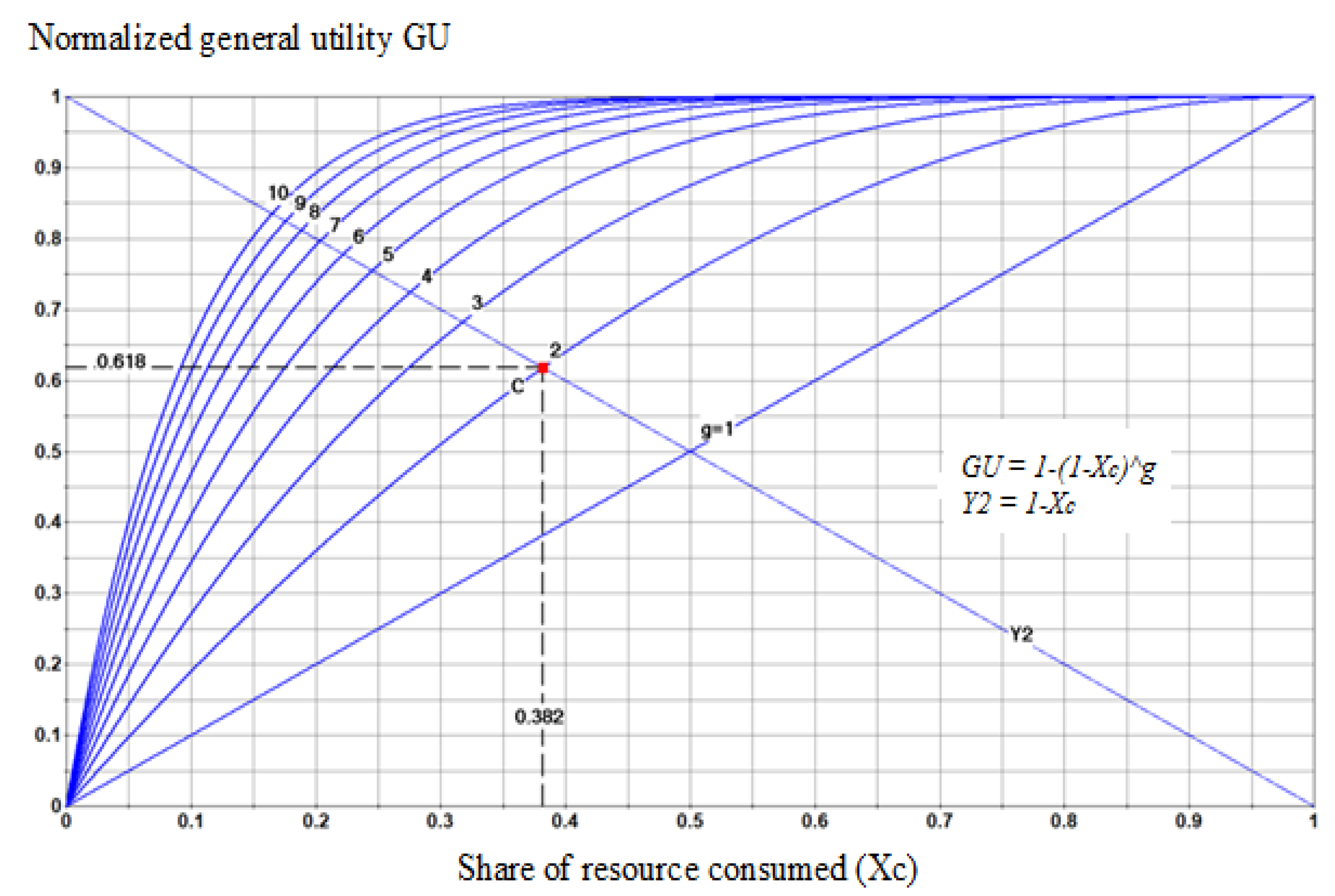
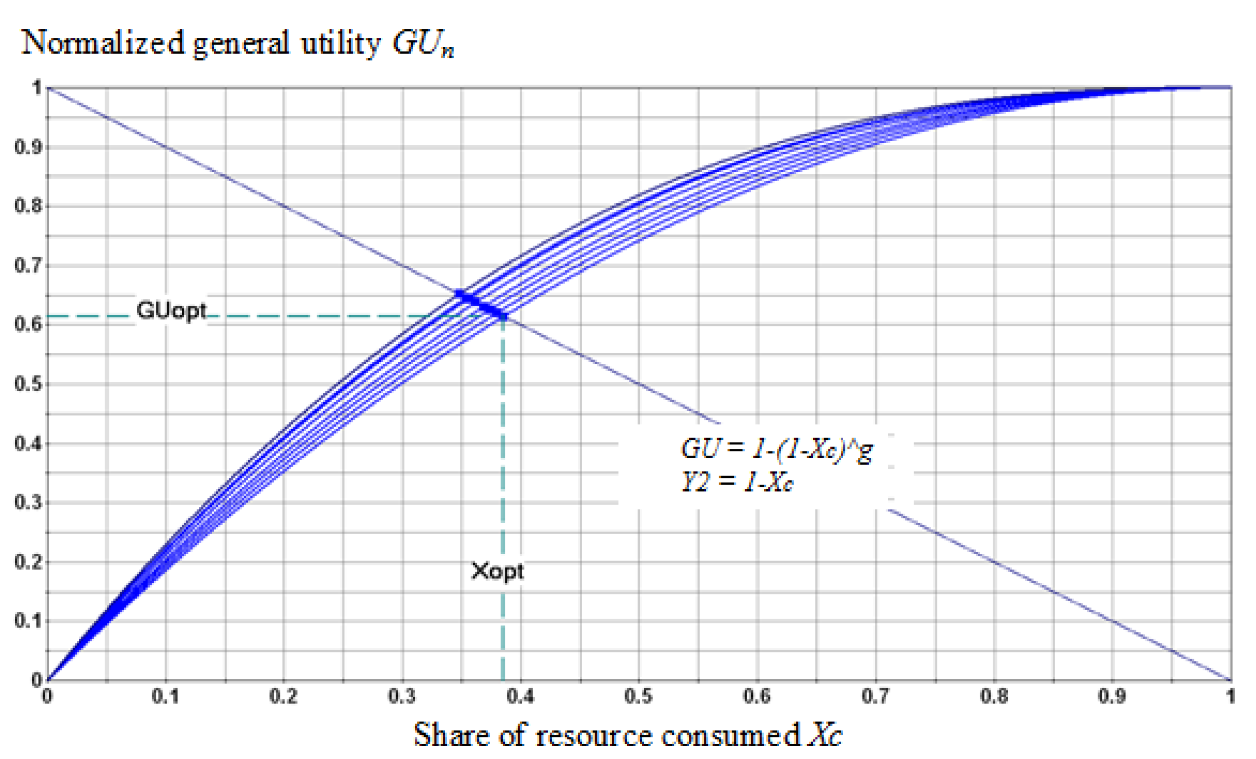
• their normalized utility function is described by the Equation (3):

  $$G{U}_n^{}=1-{\left(1-x\right)}^g$$

  (3)

  where
  • GU— the normalized general utility;
  • x—the share of consumed resource;
  • g = 1 + s—Q-factor-system quality indicator;
  • s—the multiplicity parameter, independent of x.
• they have real (independent of argument x) values of the quality factor g.

3.2. Functionality of Reference System

The essence of the functionality of reference systems of urban mobility management is to deliver the general utility of GU in the consumption of the provided resource. The macro-model of the normalized general utility GU_n is represented as (3). A significant advantage of this macro-model type is that it has fractal properties. Suppose that the argument x is an analogous function of the new parameter $T_n$, i.e.,

$$x=1-{\left(1-T_n\right)}^s$$

(4)

then normalized general utility GU_n can be represented as:

$$G{U}_n(T_n)=1-{\left(1-x\right)}^g=1-{\left\{1-\left[1-{\left(1-T_n\right)}^s\right]\right\}}^g=1-{\left[{\left(1-T_n\right)}^s\right]}^g=1-{\left(1-T_n\right)}^q$$

(5)

Obviously, the new result (3) is again a fractal that has normalized time $T_n=t/T$ as an argument (here T is a lifecycle time). The creation of the new model (3) allows us to proceed to the analysis of its dynamic characteristics.

3.3. Analysis of the Dynamic Characteristics of Reference Systems’ Functionality

For the development of an algorithmic provision for road safety management systems it is necessary to have models of the basic dynamic characteristics of the information process. Article [114] is devoted to the topic of the development of such provision.

The functional scheme of the process (Figure 1) identifies dynamic models of the following process characteristics:

-

speed of the change of process utility SGU (speed of general utility):

$$SGU(T_n)=dGU(T_n)/d{T}_n$$

(6)

-

process utility GU (general utility):

$$GU(T_n)={\displaystyle \underset{0}{\overset{T_n}{\int }}SG{U}_p(T_n) · d{T}_n}$$

(7)

-

vital power (performance) of process VP (vital power):

$$VP(T_n)=GU(T_n) · SG{U}_p(T_n)$$

(8)

-

reserve of process vital power S (stamina):

$$S(T_n)={\displaystyle \underset{0}{\overset{T_n}{\int }}VP(T_n)· d{T}_n}$$

(9)

Let us introduce the normalization of the above mentioned dynamic characteristics (

Table 1. Dynamic models of system characteristics.

Model	Determination Algorithm
Normalized speed of the change of process utility SGUn	$SG{U}_n(T_n)=SG{U}_p(T_n)/SG{U}_{p \max ·}={\left(1-T_n\right)}^{q-1}$, $\mathrm{where}SG{U}_{p \max ·}=q$.	(10)
Normalized process general utility GUn	$G{U}_n(T_n)=1-{\left(1-T_n\right)}^q$	(11)
Normalized vital power (performance) of process VPn	$V{P}_n(T_n)=\frac{VP(T_n)}{V{P}_{\max }}=\frac{q·Z^{q-1}·\left(1-Z^q\right)}{{\left(\frac{q-1}{2q-1}\right)}^{\frac{q-1}{q}}· \frac{q^2}{2q-1}}$	(12)
Normalized reserve of process vital power Sn	$S_n(T_n)=\frac{S(T_n)}{S_{\max }}={\left[GU(T_n)\right]}^2$	(13)

).

Let us explain the models (10–13).

From the perspective of the quality of system changes management process it is preferable to have not only a high level of technology perfection (determined by the level of general utility $GU(T_n)$), but also a high growth rate $SG{U}_p(T_n)=dGU(T_n)/d{T}_n$.

In this regard, we can take as a criterion of effectiveness (vital power) of the system management process the next value (14):

$$VP(T_n)=GU(T_n)·SG{U}_p(T_n)=q·Z^{q-1}·\left(1-Z^q\right)$$

(14)

where $Z=(1-T_n)$.

From the engineering point of view the question about the extremum of vital power $VP(T_n)$ is interesting. Its maximum is reached under the condition (15):

$$dVP(T_n)/d{T}_n=0$$

(15)

The solution of the Equation (15) is (16):

$$Z_{opt}={\left(\frac{q-1}{2q-1}\right)}^{\frac{1}{q}}$$

(16)

The maximum possible value of the process vital power VP is reached under the condition (17):

$$V{P}_{\max }={\left(\frac{q-1}{2q-1}\right)}^{\frac{q-1}{q}}·\frac{q^2}{2q-1}$$

(17)

The normalized value of the process vital power VP_n is determined by the algorithm (18):

$$V{P}_n(T_n)=\frac{VP(T_n)}{V{P}_{\max }}=\frac{q·Z^{q-1}·\left(1-Z^q\right)}{{\left(\frac{q-1}{2q-1}\right)}^{\frac{q-1}{q}}· \frac{q^2}{2q-1}}$$

(18)

In Table 1 model (18) is denoted as (12).

Argument $T_n{ }_{opt}$, corresponding to the maximum of effectiveness of the controlled process, is determined by (19):

$$T_{n opt}=1-Z_{opt}=1-{\left(\frac{q-1}{2q-1}\right)}^{\frac{1}{q}}$$

(19)

The reserve of vital power of population mobility management process can be interpreted as cumulative sum of vital powers on the interval $T_n$ (20):

$$S(T_n)={\displaystyle \underset{0}{\overset{T_n}{\int }}VP(T_n)·d{T}_n}={\displaystyle \underset{0}{\overset{T_n}{\int }}GU· dGU/d{T}_n· dT=}{\displaystyle \underset{0}{\overset{GU(T_n)}{\int }}GU· dGU=\frac{G{U}^2(T_n)}{2}}$$

(20)

The level of reserve of vital powers at the end of the lifecycle is (21):

$$S_{\max }={\displaystyle \underset{0}{\overset{1}{\int }}VP(T_v)·d{t}_v=}{\displaystyle \underset{0}{\overset{1}{\int }}GU·dGU/d{T}_n·dT=}{\displaystyle \underset{0}{\overset{1}{\int }}GU·dGU=\frac{1}{2}}$$

(21)

Introduction of the normalization generates model (22):

$$S_n(T_n)=\frac{S(T_n)}{S_{\max }}={\left[GU(T_n)\right]}^2$$

(22)

In Table 1 model (22) is denoted as (13).

3.4. The Research of the Structural Features of Utility Function of System Management

When analyzing the structure of general utility GU in multicomponent systems we should take into account two main points:

• the general utility GU of a complex system is an additive composition of individual functions of utility of system components;
• the general utility GU of urban mobility management is a consequence of interaction between chaotic state and orderliness of processes in this sphere.

When assessing the general utility GU of a complex system we need to identify the contribution of each component to the total success. A Pareto chart (PC) is a traditional tool for this type of analysis. It represents a cumulative function of the contribution of individual components into a total balance. As a rule, PC is approximated by a function (23):

$$PC=1-{\left(1-x\right)}^g$$

(23)

where

• x—normalized rank; x = r_i/r_max;
• r_i and r_max—correspondingly current and maximal ranks;
• $g=1+s$—Q-factor-system quality indicator;
• g and s—indicators.

Since PC is the increasing sum of “weights” of system components, it allows us to analytically deduce “weight” coefficients as (24):

$${\omega }_i=P{C}_i-P{C}_{i-1}={\left(1-\frac{i-1}{n}\right)}^g-{\left(1-\frac{i}{n}\right)}^g$$

(24)

Essentially, the normalized Pareto chart also represents the function of general utility GU, where x is a share of the consumed resource. A comparison of models (3) and (23) indicates their functional equivalence PC(x) = GU(x).

Found “weight” coefficients ${\omega }_i$ are used to solve two significant problems:

-

the estimation of relative structural entropy H_n [29,115,116], characterizing the level of orderliness (and structural perfection) of a process or system (25):

$$H_n=\left[-{\displaystyle \sum _{i=1}^n{\omega }_i·\ln \left({\omega }_i\right)}\right]/\ln (n)$$

(25)

-

representation of utility function GU(x) in additive form (26):

$$GU(x)={\displaystyle \sum _{i=1}^{n}G{U}_i}(x)={\displaystyle \sum _{i=1}^n{\omega }_i·\left[1-{\left(1-x\right)}^g\right]}$$

(26)

where

• $G{U}_i(x)$—an individual utility function (the share of contribution of i-component to the final system result).

Let us examine the second approach in detail.

Its specifics are generated by the wide usage in modern computer-aided manufacturing systems of F-technologies (F—Fibonacci). F-technologies exploit Fibonacci algorithms to build highly efficient and harmonic technical, socio-economic and organizational systems. One of the leading experts in this sphere is E. M. Soroko [29,115,116]. He found that in the majority of situations the principle of generalized golden ratio (GGR) works when the proportion between parts of the unit interval f_r and f_s (meeting the condition of normalization $f_r+f_s=1$) is right (27):

$${\left(1/f_r\right)}^s=\left(f_r/f_s\right)=f_r/\left(1-f_r\right)$$

(27)

From (27) it follows, that (28):

$$f_r^g+f_r-1=0$$

(28)

where

• $f_r$—dominant;
• $1-f_r=f_s$—subdominant;
• $g=1+s$—Q-factor-system quality indicator
• g and s—indicators.

The generalized golden ratio regime (GGR regime) directly relates to the functionality of reference management systems, presented as a macromodel of normalized general utility GU_n (3). Its graphic representation as Pareto chart PC(x) (taking into account equivalency PC(x) = GU(x)) is shown in Figure 2.

The GGR regime is presented in the figure as a diagonal y = (1 – x), where every point meets the condition y + x = 1. The point of intersection of the diagonal and Pareto chart (with coordinates f_s and f_r) is called the first Pareto point. We want to highlight its properties. Firstly, it complies with the GGR principle. Secondly, it is related to indicator g (system quality factor) by the correlation (29):

$$g=1+s=\frac{\ln \left(1-f_r\right)}{\ln \left(1-f_s\right)}$$

(29)

Thirdly, it is predetermined by proportion «order/chaos» in the management system. The meaning of the dominant f_r and f_s the subdominant is fundamentally important. The approach, evaluating levels of orderliness and chaos in an informational metric, where the maximal relative entropy of combination is taken as a unit, is foundational. The use of such approach allowed the creation of the theory of systems harmony [29]. However, at the same time, there is some non-transparency of the harmony concept in terms of engineering of efficient systems of urban mobility management. Let us consider the methodology of the optimal synthesis of harmonic systems in the examined domain sphere.

If we assume that the target management function is the retention of a process at the first Pareto point, then we need to prove that it provides an optimum in terms of predetermined parameter; in our case by default it is harmony. However, the harmonicity concept is not clearly formalized yet, and the question of an acceptable metric remains open. It is obvious that the total process utility in the first Pareto point is higher, the larger value of parameter g. However, the choice of the optimal value of the indicator g is not simple. With a decline in the value of indicator g, system losses should increase due to the poor quality of the system. With the growth of the indicator g the system efficiency should increase and, as a consequence, the additional expenses on the implementation of a system’s functioning would grow. This problem belongs to the optimization category, where we need to establish which conditions provide minimal total expenses Z and what is the value of the reached extremum Z_min.

The solution to this problem is given in the work [117]. A short explanation is given below.

In the paper it is supposed that the total expenses Z are caused by the simultaneous effect of two mechanisms:

• on the one hand, a low value of the indicator g indicates a low system efficiency and, as a consequence, it is related to unwanted losses Z₁;
• on the other hand, a growth of the value g is impossible withoud additional expenses Z₂.

Equation (28), written in the form $1-f=f^g$ (f – is a dominant of GGR regime), reaches a compromise. The left part characterizes the negative of decline of the f dominant, while the right part characterizes the positive, provided by its growth.

The negative $(1-f)$ leads to proportianal losses $Z_1=C_1·(1-f)$ (where $C_1$ − cost), when the positive $f^g$ demands proportional expenses $Z_2=C_2·f^g$.

Therefore total expenses are (28):

$$Z=Z_1+Z_2=C_1·(1-f)+C_2·f^g$$

(30)

It is important that the price C₁ can have a broad meaning. Price C₁ can be understood as money, energy, information, time and other resource types. The essence of article [117] consists in the fact that the harmonic regime is the regime of provision of the minimal total resource expenses in the first Pareto point.

It is established in [117] that the level of total expenses Z is (31):

$$Z=Z_{\max }·\left(1-f+m·f^g\right)$$

(31)

where $m=\frac{1}{g·f_r^{g-1}}$.

The normalized value of expenses equals to Z_n (32):

$$Z_n=Z/Z_{\max }=\left(1-f+m·f^g\right)$$

(32)

The minimum of expenses is reached under the condition $d{Z}_n/d{f}_r=0$. Value of extremum $Z_{n \min }$ equals to (33):

$$Z_{n \min }=1-f_r·\left(1-1/g\right)$$

(33)

and the level of minimal total expenses equals to (34):

$$Z_{\min }=Z_{\max }·\left[1-f_r·\left(1-1/g\right)\right]$$

(34)

3.5. Establishment of the Relation between Functionality and Structure

Associating the system functionality with the function of general utility GU, it was detected that the key characteristic of GU is the indicator g, which determines the level of success (the positive) in the consumption of the available resource and the structure of “weight” coefficients (relation (23)). However, the “weight” structure in turn predetermines the level of relative entropy H_n (25). Therefore, the relation between g and H_n is quite expected (Figure 3).

3.6. Identification of Model of Evaluation of Reference Systems’ Efficiency

The successful solution of management problems is based on competent goal-setting, the quantitative measure of which is an efficiency. Formally, efficiency is a relation of performance to the resource expenses on results’ achievement.

Let us consider the interpretation of the concept of “performance“.

Traditionally, success is associated with the dominant f_r; the higher the dominant, the more positive the result. Since f_r is a measure of the total utility, as a consequence, it can be a characteristic of the performance of the examined process. Model GU = f(g) is a useful tool for success evaluation. It indicates that the quantitative characteristic of management performance can be presented both as general utility GU and as a system (process) characteristic g, defined as a quality factor or Q-factor.

Therefore, there are two possible options for performance evaluation. Meanwhile, it is important to correctly evaluate resources expenses on the result achievement.

Analysis of efficiency of reference systems. If we define efficiency as a relation of performance to resource expenses, then we can consider two alternative options:

$$\mathrm{criterion} 1 E{F}_1=f_r/Z\to \max ,$$

(35)

$$\mathrm{criterion} 2 E{F}_2=g/Z\to \max .$$

(36)

The analysis showed that the second option, i.e., analysis of the system efficiency with regard to the criterion 2 (36), is more preferable than the first, because it provides higher elasticity EF relative to the total utility GU. The relation $E{F}_{2m}/E{F}_{1m}=g/f_r$ in the mode of the golden ratio (when $g=2$; $f_r= 0.618$) is equal to 3.23.

The plot of dependency of efficiency EF₂ on dominant f_r for reference systems (with different levels of quality factor Q-factor estimated g) is shown in Figure 4.

In the analysis of the model of process (system) efficiency, presented in Figure 4, it may seem as if the growth of the efficiency of reference systems is not limited at all. In fact, with the growth in the quality factor Q-factor estimated g, the system cost is increasing and according to the paper [118], this cost is proportional to g. Due to the high elasticity of the process efficiency relative to Q-factor estimated g, the system sustainability stock is decreasing and the possibility of bifurcation is increasing. The issue of the boundary of the efficient systems’ sustainability is quite important but it requires individual consideration.

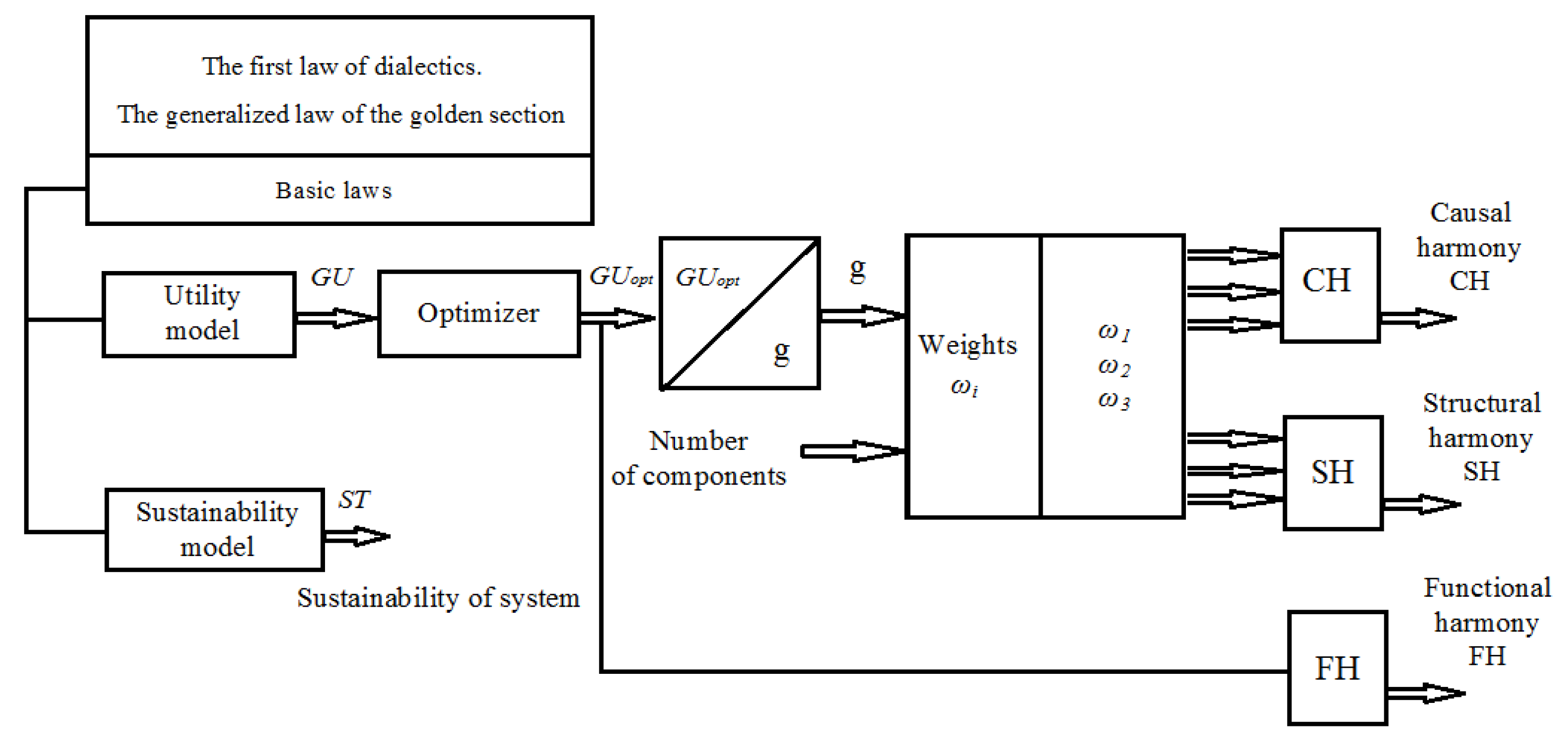
3.7. Conceptual Model of Reference System Analysis

Key properties of any rational systems are integrity and goal-orientation. System goals can differ but their main humanistic destination is a creation of some positive (utility). Management of complex systems is directed towards the growth of the positive. However, there are always forces that prevent the growth. Counteraction of multidirectional vectors forms dialectical results of complex systems’ functioning. The antagonistic force of the utility is a system’s sustainability.

With the growth of the consumed resource, the utility should increase, but at the same time the remaining resource is declining and this fact determines system sustainability and its ability to stably function. Therefore, the utility growth is not unlimited. In this situation the suggestion about some optimal (harmonious) system working mode occurs. The traditional approach supposes hidden (latent) work of some global mechanism, called the golden ratio or golden mean.

Lately the principle of the general golden ratio (GGR), established by Belarusian scientist E. M. Soroko [29] started to be used for analysis. Researchers of the V.A. Trapeznikov Institute of Management Problems of the Russian Academy of Science [119,120] created new scientific field: F-technologies (F—Fibonacci), successfully solving complex application problems of efficient management in the systems of various purposes.

The conceptual model (Figure 5) that we use also relies on the GGR principle and the first dialectic law. This model defines two new entities: normalized total utility and normalized sustainability.

The research into these characteristics allows us to solve two important problems: the problem of the optimization of the system utility GU and the problem about the logical consequences generated by this optimization (casual, structural and functional system harmonies).

3.8. Definition of the System Utility Function

The system utility is characterized by the level of system functionality. Analytically it is set by the model of total utility GU.

In the structural identification of this model, we will assume that the first dialectic law works:

Positive + negative = universum.

We interpret the positive as a saved resource and the negative as an under-received utility. After normalization we have

$$a + b=1$$

where

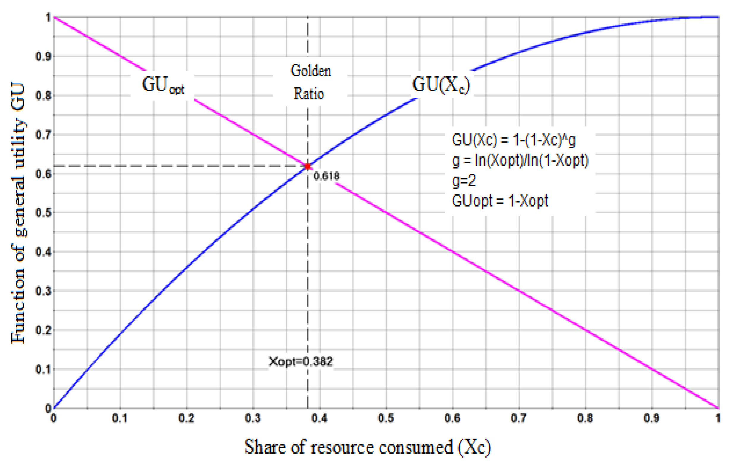
• a—dominant, a = 1 − x_c;
• x_c—the share of resource consumed on goal achievement;
• b—subdominant; b = 1 − GU;
• GU—the share of received utility relatively to maximal possible.

The GGR principle works as follows:

$${\left(\frac{1}{a}\right)}^s=\frac{a}{b}$$

which gives (37):

$${\left(\frac{1}{1-x_c}\right)}^s=\frac{1-x_c}{1-G{U}_n}$$

(37)

i.e.,

$$G{U}_n (x_c)=1-{\left(1-x_c\right)}^g$$

(38)

where

• g—Q-factor-system quality indicator.

The plots of total utility functions for different values of the quality control g are presented on Figure 6.

In Figure 6 the point C, corresponding to the classical golden ratio (under the condition g = 2), is highlighted. All sustainable solutions, conformed to GGR, are placed on the diagonal $Y_2=1-x_c$.

The analysis of extremely possible utility PU (37) showed that GU meets the necessary requirements, i.e., it declines with the growth of consumed resource $x_c$ (39):

$$PU=dGU/d{x}_c=g·{\left(1-x_c\right)}^{g-1}$$

(39)

3.9. Optimization of the Total Utility (Criteria of Optimality, System Harmonization)

Taking into account the essence of the first dialectic law, we should expect a confrontation between the system positive and the system negative. The sustainable balance between them forms the system balance. Many authoritative scientists [121,122,123] suppose that system balance is identical to the concept of system harmony. In that point (denoted as $x_{opt}$) two conditions should simultaneously meet:

• with regard to the first dialectic law, $a+b=1$, where $a=1-x_c$; $b=1-GU$), the next condition should be satisfied

  $$a+b=\left(1-x_c\right)+\left(1-GU\right)=1, \mathrm{i}.\mathrm{e}., GU=1-x_c.$$
• with regard to GGR, $GU=1-{\left(1-x_c\right)}^g$.
  Therefore, in the optimum point (where $x_c=x_{opt}$) we have

  $$1-x_{opt}=1-{\left(1-x_{opt}\right)}^g$$

  which implies that the quality factor equals to (40):

  $$g=\frac{\ln (x_{opt})}{\ln \left(1-x_{opt}\right)}$$

  (40)

In the regime of classical golden ration, when $g=2$, $x_{opt}=0.382$, substitution (40) into (37) gives an important result (41):

$$G{U}_{opt}=1-{\left(1-x_{opt}\right)}^{\frac{\ln (x_{opt})}{\ln \left(1-x_{opt}\right)}}=1-x_{opt}$$

(41)

Therefore,

$$G{U}_{opt}=1-x_{opt}$$

(42)

It means that:

-

optimal solutions are always placed on the diagonal (42);

-

system quality factor in the optimum point equals to $g=\frac{\ln (x_{opt})}{\ln \left(1-x_{opt}\right)}$;

-

work state in optimum should be considered as harmonious system state;

-

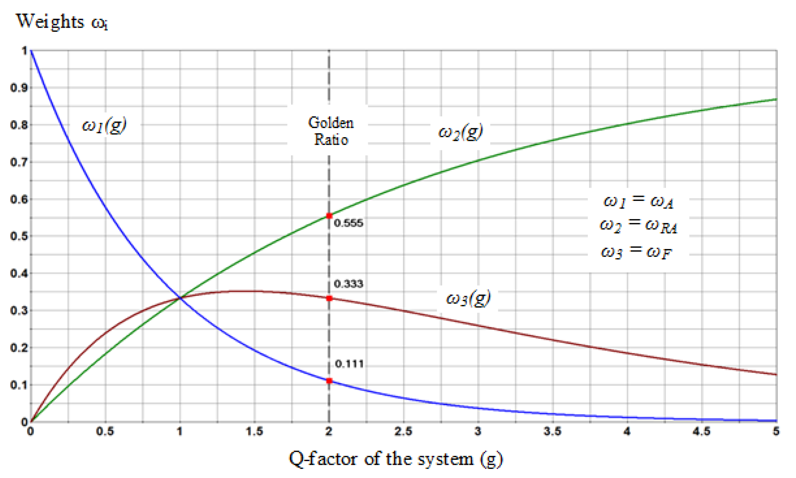
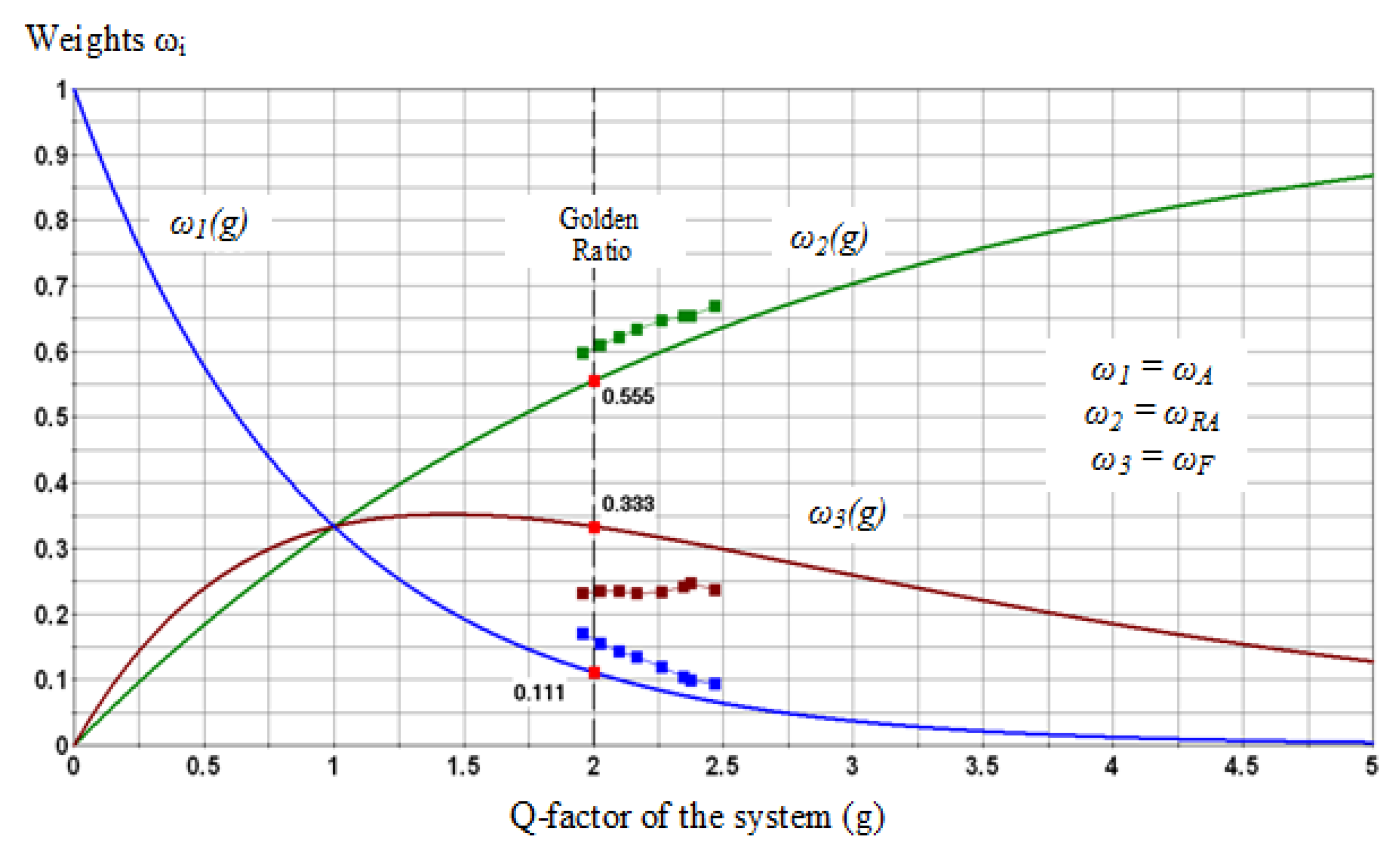
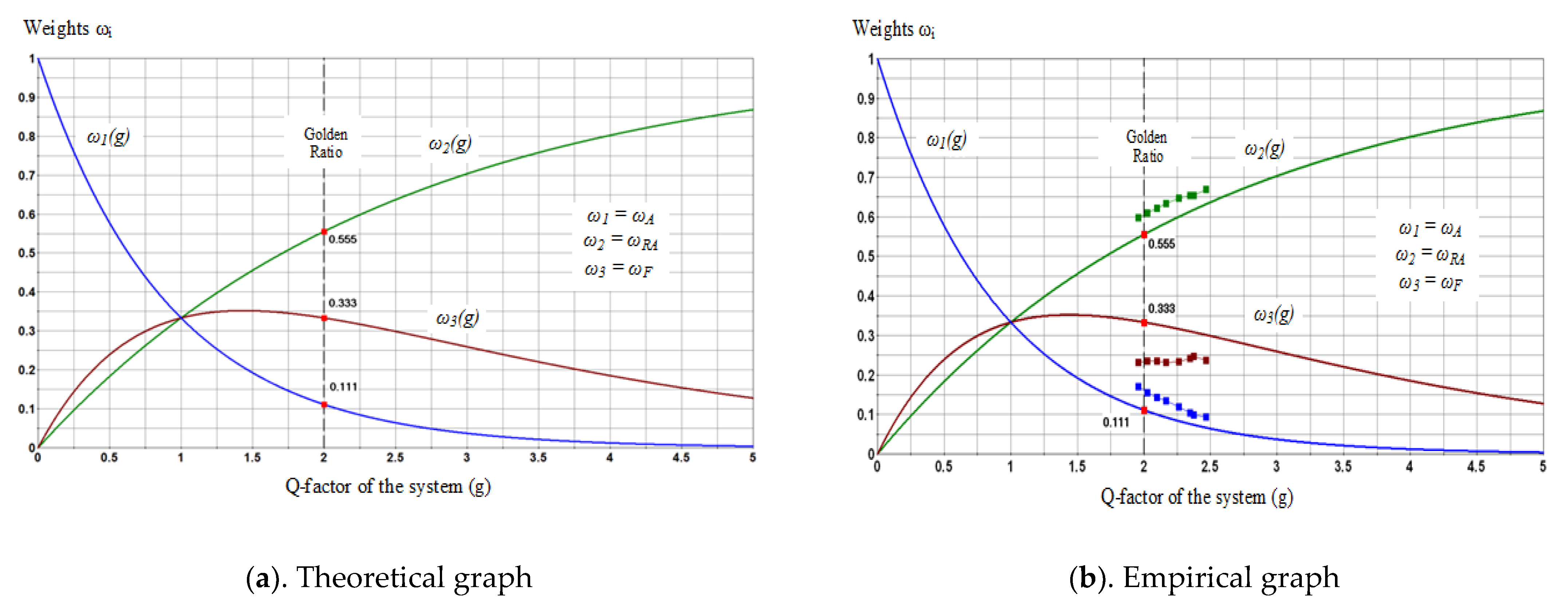
“weights” ${\omega }_i$ of system components, as shown in work [124], are predetermined by the system quality factor g (43):

$${\omega }_i={\left(1-\frac{i-1}{n}\right)}^g-{\left(1-\frac{i}{n}\right)}^g$$

(43)

where

• n—the number of components of the system under study;
• i—the rank of the component.

In the “golden ratio” regime (when g = 2) formula (41) takes the form (44):

$${\omega }_i=\frac{2}{n}-\frac{\left(2·i-1\right)}{n^2}$$

(44)

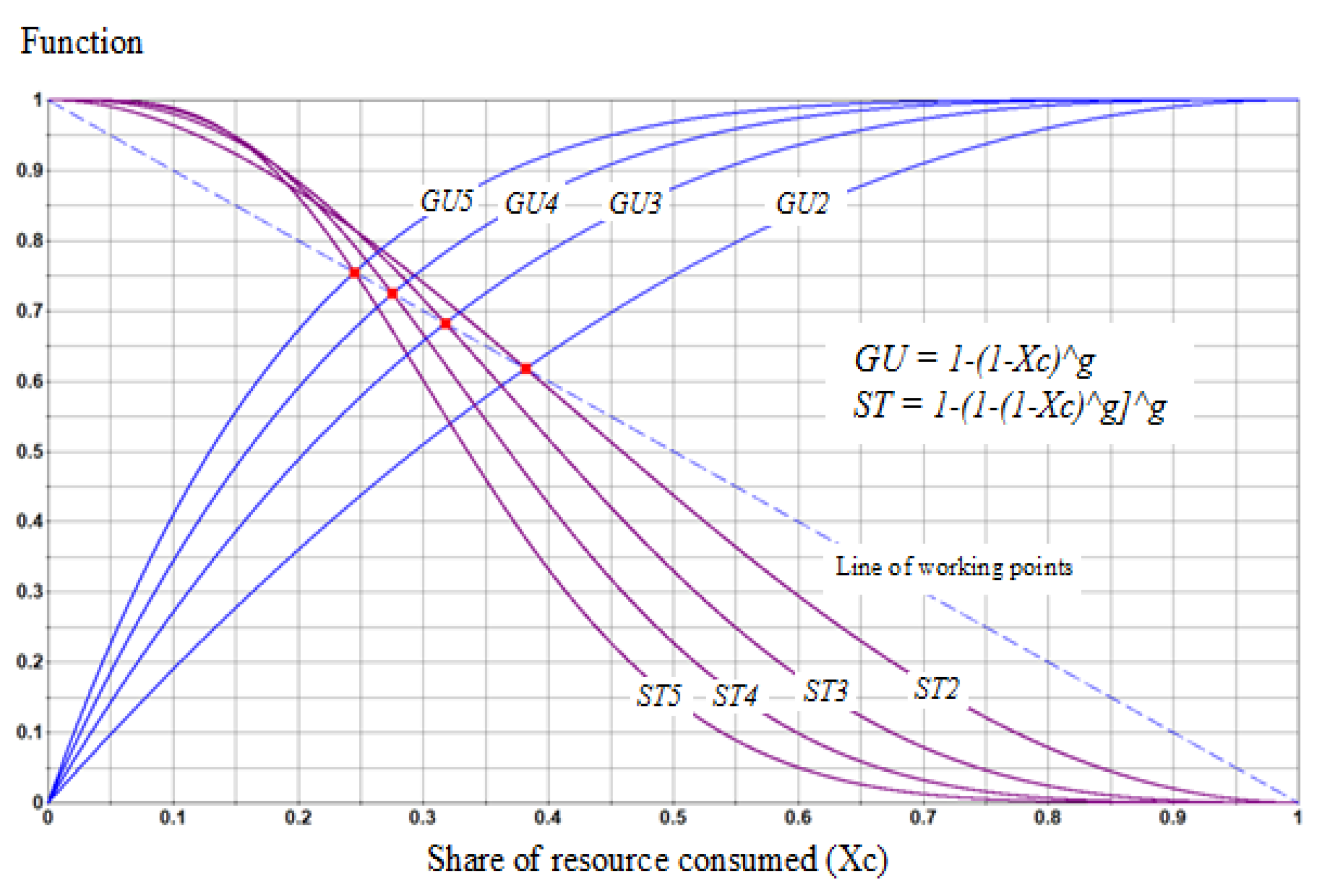
3.10. Evaluation of the Complex Systems’ Sustainability

In recent times, in strategic management publications [125] the concept of sustainability is broadly used. Different authors variously interpret this concept [126]. The majority define it only from the economic or ecological point of view, but in fact this concept has a wider meaning. There is no unified point of the view on this issue yet. At the same time the sustainability concept is significant in system analysis. It predetermines the successfulness of functioning of an analyzed complex system.

Sustainability can be evaluated by different metrics. We will use the metric of the generalized golden ratio (GGR). As was shown earlier in Section 2.1:

Positive + negative = universum.

The positive (P) assumes the growth of system utility, while the negative (N) is defined by the loss of system sustainability.

In the growth of the system utility the first summand—the Positive (P)—is dominant and after the normalization it will take the form of GU_opt. GU_opt is total utility in the operating point. The second summand—the Negative (N)—is a subdominant and it defines the share of the lost sustainability (1 - ST_opt.); here ST_opt. is a normalized sustainability in the operating point.

We will use GGR in the form ${\left(\frac{1}{G{U}_{opt}}\right)}^s=\frac{G{U}_{opt}}{1-S{T}_{opt}}$, and as a result we will have (45):

$$S{T}_{opt}=1-G{U}_{opt}^g$$

(45)

where

• g—Q-factor-system quality indicator; g = s + 1.

Analysis of the formula (45) allows us to make a significant conclusion: The growth of the utility is not unlimited: it is restrained by the loss of the sustainability. Sustainability (as an ability to execute prescribed functionality) is defined by the remaining resource and with its decline it also declines.

3.11. Establishment of the Relation between System Sustainability and Its Utility

The relation between the sustainability and the utility in the operating point (i.e., $x_c=x_{c opt}$) is characterized by the relation (45). In points x_c the structure of this relation is inherited and the sustainability model can be represented in the form (46):

$$ST(x_c)=1-{\left[GU(x_c)\right]}^g=1-{\left[1-{\left(1-x_c\right)}^g\right]}^g$$

(46)

Plots of the functions ST(x_c) and GU(x_c) are presented in Figure 7.

Operating points, corresponding to values of the quality factor g = 2, 3, 4 and 5 are highlighted. The pair GU₂ and GT₂ belongs to the golden ratio regime (g = 2). In the operating point the condition

GU₂(x_c) = ST_c(x_c) = 0.618 is met.

3.12. Analysis of the Possibilities of System Sustainability Application

There is a series of spheres in which arises a need to evaluate the sustainability level. From the positions of the PEST analysis [125] there are several types of sustainability:

• social;
• ecological;
• economic;
• technological (energetical);
• political.

In cases of sustainable urban mobility development, we should use vector (generalized) sustainability evaluation (47):

$$ST={\displaystyle \sum _{i=1}^n{\omega }_i}·S{T}_i$$

(47)

where

• ST_i—sustainability in thei-sphere;
• ${\omega }_i$—the “weight” coefficients, meeting the normalization condition ${\displaystyle \sum _{i=1}^n{\omega }_i=1}$.

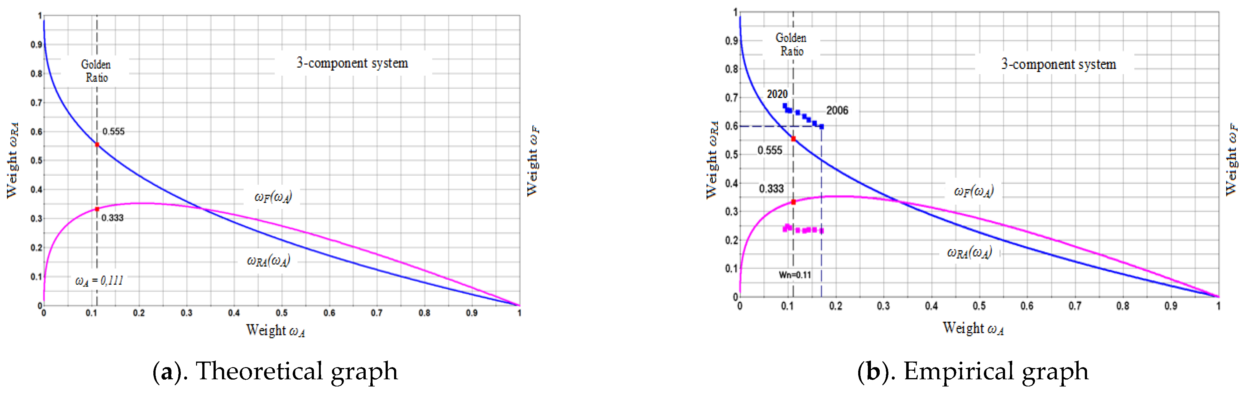
3.13. Harmonization of Complex Systems

Usually, harmony is considered from three points of view [29]. Firstly, it is considered from the positions of the character and mechanism of harmonious impact of one system part on another (casual harmony). Secondly, it is considered as proportionality of the parts in the whole (structural harmony). Thirdly, it is considered as the mutual consistency and synchronicity of system components functioning (functional harmony). The authors agree with E. M. Soroko’s point of view [29,115,116,117], consisting of the observation that system harmony is observed in the regime of the classical golden ratio, when the system quality factor equals g = 2.

4. Identification of the Q-factor g of the Road Safety Provision System

4.1. The System Orderliness and Its Relation to the System Quality Factor

In Section 2.1 it was shown that the base of the system orderliness is the structural sustainability. Maintenance of the system structural sustainability in the conditions of the negative impact of chaos is a consequence of the high level of the system orderliness. The system orderliness is identified by the features of the “weight” distribution Pareto charts or the system/process elements’ significance in the formation of the system functioning result. It is quantitatively evaluated by the level of the curvature of the Lorenz curve of the Pareto chart.

The normalized Pareto chart is presented as a function of the normalized generalized utility GU_n, where x is the share of the used resource (Equation (1)). As it was shown above in Section 3.4, the Pareto chart is an increscent sum of “weights” ${\omega }_i$ of the components of the considered system. As it was shown in Equation (22), the “weight” coefficients ${\omega }_i$ are defined by the equation:

$${\omega }_i=D{P}_i-D{P}_{i-1}={\left(1-\frac{i-1}{n}\right)}^g-{\left(1-\frac{i}{n}\right)}^g$$

In addition, earlier in Section 2.1, in Equation (23) it was presented that the found “weight” coefficients ${\omega }_i$ relative structural entropy $H_n$, characterizing the level of orderliness (or structural perfection) of the process or the system:

$$H_n=\left[-{\displaystyle \sum _{i=1}^n{w}_i·\ln \left({\omega }_i\right)}\right]/\ln (n)$$

The utility function GU(x) in the additive form can be presented as the sum of particular utility functions (or the sum of the shares of the contribution of i-components in the system result) (48):

$$GU(x)={\displaystyle \sum _{i=1}^{n}G{U}_i}(x)={\displaystyle \sum _{i=1}^n{\omega }_i·\left[1-{\left(1-x\right)}^g\right]}$$

(48)

In this equation, x is a share of the used resource and g identifies the system quality factor. The determination of the relative structural entropy $H_n$ is important from the positions of the identification of the level of the system orderliness and the system quality factor g.

4.2. Method of Definition of Relative Entropy of Road Safety Provision System

Formula (41) connects “weights” ${\omega }_i$ of researched system components and the quality factor g. Consequently, this raises the question of the system itself, its components, their “weights” and the relative importance of each component to the formation of the system functioning result.

To consider the road safety provision system we need to define the size of the system (federal, regional, district, urban or microdistrict) and the cause-and-effect relationship of road accident rate formation.

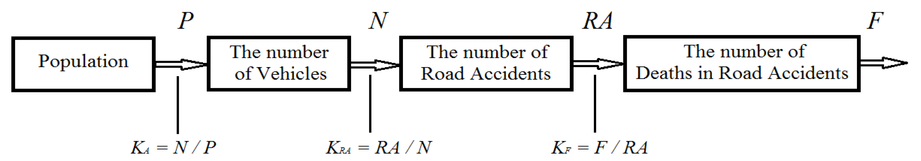
4.2.1. The Cause-and-Effect Model of Road Accident Rate Formation

The cause-and-effect model for a road safety provision system is shown in Figure 8.

The goal of the analysis of the cause-and-effect model (Figure 8) is to establish the relationship between coefficients of the informational transfer of elements of the road accident rate formation process.

For the research into the examined process structure, we will use cybernetic modeling. The concept of cybernetic modeling is defined by V.I. Krutov et al. [127] in the following way: “cybernetic models are based on the receiving of relations between input and output function for some black box or grey box, representing examined an phenomenon, without disclosure of its inner structure”.

We should pay attention not to the inner mechanism of each component of the examined process chain but only to coefficients K_i of the informational transfer between elements of the cause-and-effect model. K_i plays a special role in the analysis of the process model. It comprises the key characteristics of the elements of the complex system, the model of which is entirely defined by the behavior of its elements. The coefficient of the transfer of the i-element of the cause-and-effect model is a relation between its output (A_out) and input (A_in):

$$K_i=A_{out}/A_{in}$$

With regard to the structure of the road accident rate mechanism (Figure 8) we distinguish 3 subprocesses:

• the formation of the vehicle fleet, determining the average annual intensity of road traffic (with the transfer coefficient $K_A=N/P$);
• the formation of the road accidents (with the transfer coefficient $K_{RA}=RA/N$);
• the formation of the deaths rate in road accidents, the number of the deceased in road accidents (with the transfer coefficient $K_F=F/RA$);

4.2.2. Determination of the Priorities of the Process Elements (ABC Analysis)

The ABC analysis, based on the Pareto chart, is a tool of determination of the priorities of the examined process elements. The aim of the analysis is to identify main priorities. The essence of the ABC analysis consists of the search for the first and the second Pareto points (determining the position of the boundaries between A, B and C areas).

To hold this analysis, it is necessary to preliminarily make a decision on 3 issues: decide what to define as the positive; choose necessary metric; prepare data.

For the first problem, it is obvious that the lower the transfer coefficient K of the element, the more positive the result. Generally, for the whole cause-and-effect process chain we can say that the lower the value of the through transfer coefficient K_i, the more positive the system result.

In the next step we need to learn how to measure the positive, i.e., introduce the necessary metric. It is reasonable to use an indicator of the process Q positive as a measure (49):

$$Q_i=\ln \left(1/K_i\right)$$

(49)

Received results allow us to find “weak“ elements in the chain of the cause-and-effect relations in the road accident rate formation process and set priorities in the road safety management sphere.

4.2.3. Evaluation of the “Weight” Coefficients ${\omega }_i$

Knowing the values of the positive of process elements Q_i, we determine the total process positive Q (50):

$$Q=Q_A+Q_{RA}+Q_F=\ln \left(1/K_A\right)+\ln \left(1/K_{RA}\right)+\ln \left(1/K_F\right)$$

(50)

The “weight” coefficients ${\omega }_i$ show the share of each summand $Q_i$ in the total sum of the process positive Q (51):

$${\omega }_i=\frac{\ln \left(1/K_i\right)}{{\displaystyle \sum _{i=1}^3\ln \left(1/K_i\right)}}$$

(51)

4.2.4. Evaluation of the Entropy as A Characteristic of the Orderliness of the Road Safety Provision System

The structure of the “weight” coefficients ${\omega }_i$ of the road safety provision process defines the level of the orderliness. The numerical characteristic of the orderliness level is an entropy H (52):

$$H=-{\displaystyle \sum _{i=1}^n{\omega }_i}·\ln {\omega }_i$$

(52)

where

• n—the number of system elements (in our case n = 3);
• ${\omega }_i$—the “weight” coefficients, meeting the normalization condition ${\displaystyle \sum _{i=1}^n{\omega }_i=1}$.

Relative entropy H_n is more visual and convenient from the positions of the application characteristic of the evaluation of the road safety provision system’s orderliness (53):

$$H_n=H/\ln (n)$$

(53)

where

• n—the number of system elements (in our case n = 3);

From now on we will use this characteristic to evaluate the orderliness of the road safety provision systems.

4.3. The Method of the Determination of the Quality Factor of the Road Safety Provision System

As was shown in Section 2.4 and Section 4.1, value g is an exponent of the exponential equation, identifying the curvature of the change in the Pareto chart cumulate. Equation (27), presented in Section 3.4, illustrates the meaning of the system quality factor g:

$$g=1+s=\frac{\ln \left(1-f_r\right)}{\ln \left(1-f_s\right)}$$

By knowing the coordinates $f_r$ and $f_s$ of the curve, which identify the utility function GU(x), we can determine the value of the quality factor of the system.

5. Example of the Theoretical Solution of the Problem of the Evaluation of the System Harmonicity in Relation to the Road Safety Provision System

As an example, we will provide results of the harmonic analysis of the complex systems in the road safety sphere, one of the key spheres of the urban mobility implementation. In this analysis the results of the authors’ research relied on the database of the State Inspectorate for Road Traffic Safety [11].

The three “weight” coefficients of the rank Pareto chart are the subject of the analysis: “weight”, characterizing the level of automobilization (${\omega }_A$); “weight”, characterizing the level of road accidents (${\omega }_{RA}$) and “weight”, characterizing the death rate (${\omega }_F$). The sum of “weights” meets the normalization condition ${\displaystyle \sum _{i=1}^3{\omega }_i}=1$

5.1. Structural Harmony

In reference systems, the “weight” coefficients are always determined (see relation (43), Figure 9).

In the golden ratio regime, when g = 2, components’ “weights” (Figure 9) correspond to the proportions (44) and when n = 3 they are correspondingly equal: ${\omega }_A=0.111$; ${\omega }_{RA}=0.555$; ${\omega }_F=0.333$.

5.2. Casual Harmony

In the analysis it was taken into account that the level of automobilization A is the root cause, while the number of road accidents and the number of deceased in road accidents are consequences of the automobilization A. Therefore, it is reasonable to present the casual harmony in the form of the dependency of the “weights” ${\omega }_{RA}$ and ${\omega }_F$ on the “weight” ${\omega }_A$ (Figure 10).

The relation of the “weights” is of practical interest. It is presented in Figure 11.

5.3. Functional Harmony

According to Socrates [29], we connect functional harmony with the utility principle. The optimal level of the normalized utility is observed in the golden ratio conditions (Figure 12) and it is equal to 0.618.

6. Quantitative Assessment of Changes in the Road Safety System Harmonicity in the Russian Federation

6.1. Assessment of the General Trend in Changes in the Road Safety System Harmonicity in Russia from 2006 to 2020

The data source was the official statistics of the State Inspectorate for Road Traffic Safety of the Russian Federation [11]. Over the past 15 years (2006–2020), the indicators of road safety in Russia have been constantly improving. A number of factors have contributed to this, such as a general increase in the transport culture of the country’s population, a significant increase in the quality of the country’s transport fleet and significant qualitative growth of the country’s road transport infrastructure. It is also important that since 2006, a lot of attention has been paid to the issues of road safety provision by the Russian government [9,10].

The result of the improvement in the overall situation in the transport sphere was a decrease in the annual number of accidents and deaths in road accidents in Russia over the past 15 years (

Table 2. Changes in the main road safety indicators in the Russian Federation from 2006 to 2020.

Road Safety Indicators	Numerical Values of Indicators By Year
	2006	2008	2010	2012	2014	2016	2018	2020
Number of accidents, units	228,309	217,557	199,083	203,597	199,720	173,694	168,099	137,662
The number of people killed in accidents, deceased people	32,724	29,936	26,567	27,991	26,963	20,308	18,214	15,788

).

The natural result of a long-term decrease in road traffic accident rate in Russia was a significant decrease in the relative entropy H_n of the road safety system and an increase in its Q-factor g (

Table 3. Changes in relative entropy H_{n RSS} and Q-factor g values of the road safety system in Russia.

Characteristic	Numerical Values of Indicators By Year
	2006	2008	2010	2012	2014	2016	2018	2020
Relative entropy of the road safety system Hn RSS	0.862	0.847	0.831	0.817	0.797	0.780	0.775	0.755
Q-factor of the road safety system g	1.956	2.027	2.098	2.166	2.262	2.346	2.374	2.465

).

The dynamics of the change in Q-factor g of the road safety system of the Russian Federation from 2006 to 2020 is very impressive.

At the same time, the ratio of “weight” coefficients ${\omega }_i$ changes over time. Based on these dynamics, it is possible to estimate changes in all three types of system harmony: structural, causal and functional.

Let us consider the actual data characterizing the “weight” coefficients ${\omega }_i$, and draw conclusions about the dynamics of the road safety system harmony in Russia over the past 15 years (2006–2020).

Table 4. Changes in the numerical values of the “weight“ coefficients ${\omega }_i$ from 2006 to 2020.

Characteristic	Numerical Values of Indicators By Year
	2006	2008	2010	2012	2014	2016	2018	2020
${\omega }_A$	0.170	0.155	0.143	0.134	0.120	0.104	0.098	0.093
${\omega }_{RA}$	0.598	0.610	0.622	0.633	0.647	0.654	0.655	0.670
${\omega }_F$	0.232	0.235	0.235	0.232	0.233	0.242	0.247	0.237

presents data on the change in the numerical values of the “weight” coefficients ${\omega }_i$ from 2006 to 2020.

Figure 13 shows the graphs of the dynamics of the “weight” coefficients of the road safety system in Russia from 2006 to 2020.

Figure 14 shows a comparison of the theoretical and actual dynamics of changes in the “weight” coefficients ${\omega }_i$ of the road safety system in Russia over a 15-year period.

The analysis of the dynamics of the values of the weight coefficients ${\omega }_i$ allows us to conclude that the value of “weight” ${\omega }_A$ has decreased almost by half over the past 15 years, the value of “weight” ${\omega }_{RA}$ has increased by 12%, and the value of “weight” ${\omega }_F$ has increased by 6% from 2016 to 2018. However, in 2020, the “weight” ${\omega }_F$ significantly dropped again. This happened due to a significant increase in the severity of road accidents in 2020. The reason is the increase in the speed of vehicle movement in Russia in 2020 in the conditions of a relative rarefaction of the traffic flow associated with pandemic restrictions on the population mobility.

This is also evidenced by the statistics of penalties for violating the requirements of traffic rules and the share of those that fall on violation of the requirements of the speed limits (

Table 5. General statistics of penalties for violators of traffic rules in Russia (2016–2020).

Indicator	Numerical Values of Indicators By Year
	2016	2017	2018	2019	2020
The number of penalties, mln. units	87.1	108.7	131.3	142.1	167.0
Of these, for violation of the speed limit, mln. units	54.0	74.4	92.2	101.8	124.0
The share of speed limit violations in the total number of violations, %	62.0	68.4	70.2	71.6	74.2

).

The data analysis in Table 5 shows that over the past 5 years in Russia, not only the number of penalties for violating traffic rules, but also the share of speed violations has increased. This indirectly indicates an increase in the quality of Russian roads and an improvement in the system of monitoring the speed limits of traffic flows. It is known that at the end of 2020, about 19,000 automated complexes for photo-video recording of traffic violations by drivers were used in Russia.

Figure 15 shows a comparison of the theoretical and actual dynamics of causal harmony of the road safety provision system in Russia over a 15-year period.

The functionality of the road safety system is estimated by the ratio of the actual level of normalized functional utility $G{U}_n$ and the share of consumed resource $X_c$, and is actually identified by the coordinate of the first Pareto point on the graph $G{U}_n=f(X_c)$.

Table 6. Changes in the numerical values of the normalized general utility $G{U}_n{ }_{RSS}$ of the Russian RSS from 2006 to 2020.

Characteristic	Numerical Values of Indicators By Year
	2006	2008	2010	2012	2014	2016	2018	2020
Normalized general utility $G{U}_{n RSS}$	0.615	0.620	0.626	0.631	0.639	0.644	0.646	0.652

shows the data on changes in the numerical values of the actual level of the normalized functional utility $G{U}_n{ }_{RSS}$ of the Russian road safety provision system.

Figure 16 shows the dynamics of the actual numerical values of the normalized general utility $G{U}_n{ }_{RSS}$ of the Russian road safety provision system from 2006 to 2020.

Comparing the data in Figure 16 with the known optimal value of the normalized utility $G{U}_{opt}=0.618$, it is easy to conclude about the current state of the Russian road safety provision system harmonicity.

6.2. Comparison of the Road Safety System Harmonicity in Russia during the COVID Restriction Period (2020) and during the Pre-COVID Period (2019)

COVID-restrictions on mobility of all types (pedestrian, transport and general) have very seriously affected the change in all characteristics that define the process of road traffic accident formation in Russia.

Table 7. Numerical values of the characteristics of the causal path of road traffic accident formation in Russia before (2019) and during (2020) the COVID-19 pandemic.

Year	Population of Russian Federation (on 1 January the Following Year), People	The Average Annual Number of the Fleet of Vehicles of the Russian Federation, Units	Annual Number of Road Accidents in the Russian Federation, Case/Year	The Annual Number of Deaths in Road Accidents in the Russian Federation, Deceased/Year
2019	146,748,590	61,739,156	164,358	16,981
2020	146,171,015	62,721,765	137,662	15,788
Absolute change, unit
Δ2020/2019	−577,575	+982,609	−26,696	−1193
Relative change, %
Δ2020/2019, %	−0.39	+1.59	−16.25	−7.02

presents data describing the process of road accident rate formation in Russia in 2019 and 2020.

Table 8. Intermediate and final results of calculating the relative entropy H_{n RS SRF} of the Russian road safety system in 2019.

Numerical Values of the Elements of the Three-Link Mechanism of Informational Transformation of the Road Safety System in the Russian Federation, 2019
Y1 – Country population	Y2 – Size of vehicle fleet	Y3 – Annual number of road accidents	Y4 – Annual number of deaths in road accidents
146,748,590	61,739,56	164,358	16,981
$K_i$ numerical values
KA	KRA		KF
61,739,156/146,748,590 = 0.4207	164,358/61,739,156 = 0.0026		16,981/164,358 = 0.1033
$\mathrm{Numerical} \mathrm{values} \mathrm{of} \mathrm{the} \mathrm{positive} Q_{\mathrm{i}}=\ln \left(1/K_i\right)$
0.8658	5.9286		2.2700
$\mathrm{Numerical} \mathrm{values} \mathrm{of} \mathrm{relative} “\mathrm{weight}” \mathrm{of} \mathrm{the} \mathrm{positive} {\omega }_{\mathrm{i}}(Q_i)$
0.096	0.654		0.250
$\mathrm{Numerical} \mathrm{values} ( \ln {\omega }_i)$
−2.3485	−0.4246		−1.3846
$\mathrm{Numerical} \mathrm{values} ({\omega }_i · \ln {\omega }_i)$
−0.2243	−0.2777		−0.3467
Numerical value of absolute entropy H RSS RF = 0.8487
Numerical value of relative entropy Hn RSS RF = 0.7726

and

Table 9. Intermediate and final results of calculating the relative entropy H_{n RSS RF} of the Russian road safety system in 2020.

Numerical Values of the Elements of the Three-Link Mechanism of Informational Transformation of the Road Safety System in the Russian Federation, 2020
Y1 – Country population	Y2 – Number of vehicle fleet	Y3 – Annual number of road accidents	Y4 – Annual number of deaths in road accidents
146,171,015	62,721,765	137,662	15,788
$K_i$ numerical values
KA	KRA		KF
62,721,765/146,171,015 = 0.4291	137,662/62,721,765 = 0.0022		15,788/137,662 = 0.1147
$\mathrm{Numerical} \mathrm{values} \mathrm{of} \mathrm{the} \mathrm{positive} Q_{\mathrm{i}}=\ln \left(1/K_i\right)$
0.8461	6.1217		2.1656
$\mathrm{Numerical} \mathrm{values} \mathrm{of} \mathrm{relative} “\mathrm{weight}” \mathrm{of} \mathrm{the} \mathrm{positive} {\omega }_{\mathrm{i}}(Q_i)$
0.093	0.670		0.237
$\mathrm{Numerical} \mathrm{values} ( \ln {\omega }_i)$
−2.34791	−0.4001		−1.4393
$\mathrm{Numerical} \mathrm{values} ({\omega }_i · \ln {\omega }_i)$
−0.2204	−0.2682		−0.3413
Numerical value of absolute entropy H RSS RF = 0.8298
Numerical value of relative entropy Hn RSS RF = 0.7553

present the intermediate (according to the methodology of Section 4.2 of the article) and final results of calculating the relative entropy of the Russian road safety system H_{n RSS RF} in 2019 and 2020.

On the basis of the numerical values of H_{n RSS RF-2019} = 0.7726 and H_{n RSS RF-2020} = 0.7553 we determined the appropriate Q-factor levels of the road safety system for the versions of 2019 and 2020.

Q-factor of the road safety system in the Russian Federation in 2019 g _{RSS RF-2019} = 2.3754, and its analogue for 2020 g _{RSS RF-2020} = 2.4646.

The calculations show that the changes in the Russian road safety system that occurred during COVID restrictions (2020) ensured a decrease in its relative entropy H_n by 2.24%, from H_{n RSS 2019} = 0.7726 to H_{n RSS 2020} = 0.7553. The orderliness of the road safety system in Russia has improved.

The Q-factor of the Russian road safety system g _RSS increased by 3.75% during COVID restrictions (2020).

Normalized general utility GU_{n RSS} increased by 0.46% from 2019 to 2020 (GU_{n RSS 2019} = 0.649 and GU_{n RSS 2019} = 0.652).

7. Conclusions

During the research it was established that the Q-factor g of the Russian road safety provision system changed from g ₂₀₀₆ = 1.9565 to g ₂₀₂₀ = 2.4646. This promotes the decline of the relative entropy of the Russian road safety provision system from H_{n RSS 2006} = 0.8623 to H_{n RSS 2020} = 0.7553. The deep reason for that change was the modification of the relation between “weights” or the significance of the contribution of different elements of the cause-and-effect chain in the formation of the factual level of the road accident rate in Russia in the last 15 years.

The main conclusion is that the harmonicity of the Russian road safety provision system, assessed by the normalized functional general utility GU_n, has been increased and it already exceeded the level of harmonious reference systems GU_n = 0.618.

Actually, the normalized functional general utility GU_{n RSS} of the Russian road safety provision system increased from GU_{n RSS 2006} = 0.615 to GU_{n RSS 2020} = 0.652 (by 6.0%) from 2006 to 2020. Simultaneously, the share of the normalized used resource X_n declined. That allowed us to make a conclusion about a significant improvement in the balance “efficiency-quality” of the Russian road safety provision system. The COVID lockdown played a positive role in this process. The harmonicity of the Russian road safety provision system, assessed by the normalized general utility GU_{n RSS}, increased by 0.46% from 2019 to 2020.

It is important to note that the methodology of the quantitative assessment of the system harmonicity can be applied to a variety of spheres of human activity. The road safety system is just one example. Exactly the same calculations can be carried out to assess the harmonicity of the functioning of a variety of socio-technical and socio-cultural systems.

References

1. Schwab, K.; Malleret, T. COVID-19. The Great Reset; World Economic Forum: Cologny, Geneva, 2020; 212p. [Google Scholar]
2. TomTom Traffic Index. Available online: https://www.tomtom.com/en_gb/traffic-index/ (accessed on 9 August 2021).
3. Sharifi, A.; Khavarian-Garmsir, A.R. The COVID-19 pandemic: Impacts on cities and major lessons for urban planning, design and management. Sci. Total Environ. 2020, 749, 142391. [Google Scholar] [CrossRef]
4. Rutz, C.; Loretto, M.C.; Bates, A.E.; Davidson, S.C.; Duarte, C.M. COVID-19 lockdown allows researchers to quantify the effects of human activity on wildlife. Nat. Ecol. Evol. 2020, 4, 1156–1159. [Google Scholar] [CrossRef]
5. Road Safety Annual Report. 2020. Available online: www.itf-oecd.org/road-safety-annual-report-2020 (accessed on 10 August 2021).
6. Resolution A/RES/74/299. Improving Global Road Safety. Available online: un.org›pga/74—uploads—Resolution-Road-Safety.pdf (accessed on 10 August 2021).
7. Voas, R.B.; Fell, J.C.; McKnight, A.S.; Sweedler, B.M. Controlling Impaired Driving Through Vehicle Programs: An Overview. Traffic Inj. Prev. 2004, 5, 292–298. [Google Scholar] [CrossRef]
8. Amador, L.; Willis, C.J. Demonstrating a Correlation between the Maturity of Road Safety Practices and Road Safety Incidents. Traffic Inj. Prev. 2014, 15, 591–597. [Google Scholar] [CrossRef]
9. Mayorov, V.I.; Sevryugin, V.E. International experience of developing complex target programs of road users’ safety. Criminol. J. Baikal Natl. Univ. Econ. Law 2015, 9, 766–776. (In Russian) [Google Scholar] [CrossRef]
10. Decree of the Government of the Russian Federation of 8.01.2018, No 1-r, On Approval of the Road Safety Strategy in the Russian Federation for 2018–2024. Available online: https://docs.cntd.ru/document/556323639 (accessed on 11 August 2021).
11. The Official Website of the State Traffic Inspectorate of the Russian Federation. Indicators of the State of Road Safety. Available online: http://stat.gibdd.ru/ (accessed on 11 August 2021).
12. Benedict, R. Synergy: Some Notes of Ruth Benedict. Am. Anthropologist. New Ser. 1970, 72, 320–333. [Google Scholar]
13. Maslow, A.H. Synergy in the Society and in the Individual. J. Individ. Psychol. 1964, 20, 153. [Google Scholar]
14. Evans, P. Government action, social capital and development: Reviewing the evidence on synergy. World Dev. 1996, 24, 1119–1132. [Google Scholar] [CrossRef] [Green Version]
15. Evans, P.; Berkeley, C.A. (Eds.) State-Society Synergy: Government and Social Capital in Development; Institute for International Studies: Berkeley, CA, USA, 1996. [Google Scholar]
16. Hauert, C.; Michor, F.; Nowak, M.A.; Doebeli, M. Synergy and discounting of cooperation in social dilemmas. J. Theor. Biol. 2006, 239, 195–202. [Google Scholar] [CrossRef] [PubMed] [Green Version]
17. Jaffe, K. Quantifying social synergy in insect and human societies. Behav. Ecol. Sociobiol. 2010, 64, 1721–1724. [Google Scholar] [CrossRef]
18. Prigogine, I.; Stengers, I. Order out of Chaos: Man’s New Dialogue with Nature; A Bantam Book: Toronto, ON, Canada; New York, NY, USA; London, UK; Sydney, Australia, 1984; 349p. [Google Scholar]
19. Prigogine, I. The philosophy of instability. Futures 1989, 21, 396–400. [Google Scholar] [CrossRef]
20. Nicolis, G.; Prigogine, I. Self-Organization in Nonequilibrium Systems; John Wiley & Sons: New York, NY, USA, 1977; 491p. [Google Scholar]
21. Othmer, H.G. Self-Organization in Nonequilibrium Systems (G. Nicolis and I. Prigogine). SIAM Rev. 1982, 24, 483–485. [Google Scholar] [CrossRef]
22. Haken, H. The Science of Structure: Synergetics; Prentice Hall: New York, NY, USA, 1984. [Google Scholar]
23. Haken, H. Synergetics: An Introduction; Springer Ser. Synergetics: Berlin/Heidelberg, Germany, 1983. [Google Scholar]
24. Haken, H. Advanced Synergetics; Springer Ser. Synergetics: Berlin/Heidelberg, Germany, 1987. [Google Scholar]
25. Liening, A. Synergetics—Fundamental Attributes of the Theory of Self-Organization and Its Meaning for Economics. Mod. Econ. 2014, 5, 841–847. [Google Scholar] [CrossRef] [Green Version]
26. Yakimtsov, V.V. History and development of Haken’s synergetics. Sci. Bull. UNFU 2018, 28, 119–125. [Google Scholar] [CrossRef]
27. Kurdyumov, S.P.; Malinetskii, G.G. Synergetics-Theory of Self-Organization. Ideas, Methods, Perspectives; Nauka: Moscow, Russia, 1983; 280p. (In Russian) [Google Scholar]
28. Kurdyumov, S.P.; Malinetskii, G.G. Prologue. Synergetics and System Synthesis. Looking to the Third Millennium; Nauka: Moscow, Russia, 2002; 420p. (In Russian) [Google Scholar]
29. Soroko, E.M. Golden Sections, Processes of Self-Organization and Evolution of Systems: An Introduction to the General Theory of Harmony of Systems, 4rd ed.; Book House “Librocom”: Moscow, Russia, 2012; 264p. (In Russian) [Google Scholar]
30. Gordon, J.E. The epidemiology of accidents. Am. J. Public Health 1949, 39, 504–515. [Google Scholar] [CrossRef] [Green Version]
31. Gibson, J.J. The Contribution of Experimental Psychology to the Formulation of the Problem of Safety—A Brief for Basic Research. Behavioural Approaches to Accident Research; Assoc. for the Aid of Crippled Children: New York, NY, USA, 1961; pp. 77–89. [Google Scholar]
32. Haddon, W. The changing approach to the epidemiology, prevention, and amelioration of trauma: The transition to approaches etiologically rather than descriptively based. Am. J. Public Health 1968, 58, 1431–1438. [Google Scholar] [CrossRef]
33. Haddon, W. A logical framework for categorizing highway safety phenomena and activity. J. Trauma 1972, 12, 193–207. [Google Scholar] [CrossRef] [PubMed]
34. Haddon, W. Energy damage and 10 countermeasure strategies. J. Trauma Inj. Infect. Crit. Care 1973, 13, 321–331. [Google Scholar] [CrossRef] [PubMed] [Green Version]
35. Haddon, W. Options for the prevention of motor vehicle crash injury. Isr. J. Med. Sci. 1980, 16, 45–65. [Google Scholar]
36. Von Bertalanffy, L. General System Theory: Foundations, Development, Applications; Penguin: London, UK, 1968. [Google Scholar]
37. Johansson, R. Vision Zero—Implementing a policy for traffic safety. Saf. Sci. 2009, 47, 826–831. [Google Scholar] [CrossRef]
38. Larsson, P.; Dekker, S.W.; Tingvall, C. The need for a systems theory approach to road safety. Saf. Sci. 2010, 48, 1167–1174. [Google Scholar] [CrossRef]
39. Szymanek, A. System Approach in Road Safety Studies. Commun. Sci. Lett. Univ. Zilina 2020, 22, 201–210. [Google Scholar] [CrossRef]
40. Hughes, B.P.; Newstead, S.; Anund, A.; Shu, C.C.; Falkmer, T. A review of models relevant to road safety. Accid. Anal. Prev. 2015, 74, 250–270. [Google Scholar] [CrossRef] [Green Version]
41. Smeed, R.J. Some statistical aspects of road safety research. J. R. Stat. Soc. 1949, 12, 1–34. [Google Scholar] [CrossRef]
42. Haight, F.A. Traffic safety in developing countries. J. Saf. Res. 1980, 12, 50–58. [Google Scholar] [CrossRef]
43. Jacobs, G.D.; Cutting, C.A. Further research on accident rates in developing countries. Accid Anal. Prev. 1986, 18, 119–127. [Google Scholar] [CrossRef]
44. Nicholson, A.J.; Jadaan, K.S. A review of recent developments and current issues in road safety. J. Traffic Med. 1989, 17, 13–22. [Google Scholar]
45. Zwi, A.B.; Forjouh, S.; Murugusamphillay, S. Injuries in developing countries: Policy response needed now. Trans. R. Soc. Trop. Med. Hyg. 1996, 90, 593–595. [Google Scholar] [PubMed] [Green Version]
46. Murray, C.J.L.; Lopez, A.D. Mortality by cause for eight regions of the World: Global burden of disease Study. Lancet 1997, 349, 1269–1276. [Google Scholar] [CrossRef]
47. Bener, A.; Abu-Zidan, F.M.; Bensiali, A.K.; Al-Mulla, A.A.; Jadaan, K.S. Strategy to improve road safety in developing countries. Saudi Med. J. 2003, 24, 603–608. [Google Scholar] [PubMed]
48. Belin, M.-Å.; Tillgren, P.; Vedung, E. Vision Zero—A road safety policy innovation. Int. J. Inj. Control Saf. Promot. 2012, 19, 171–179. [Google Scholar] [CrossRef] [Green Version]
49. Haagsma, J.A.; Graetz, N.; Bolliger, I.; Naghavi, M.; Higashi, H.; Mullany, E.C.; Abera, S.F.; Abraham, J.P.; Adofo, K.; Alsharif, U.; et al. The global burden of injury: Incidence, mortality, disability-adjusted life years and time trends from the Global Burden of Disease study 2013. Inj. Prev. 2016, 22, 3–18. [Google Scholar] [PubMed] [Green Version]
50. Goniewicz, K.; Goniewicz, M.; Pawłowski, W.; Fiedor, P. Road accident rates: Strategies and programmes for improving road traffic safety. Eur. J. Trauma Emerg. Surg. 2016, 42, 433–438. [Google Scholar] [CrossRef]
51. Beck, B.; Cameron, P.A.; Fitzgerald, M.C.; Judson, R.T.; Teague, W.; Lyons, R.A.; Gabbe, B.J. Road safety: Serious injuries remain a major unsolved problem. Med. J. Aust. 2017, 207, 244–249. [Google Scholar] [CrossRef] [PubMed]
52. WHO. Available online: https://www.who.int/ (accessed on 13 August 2021).
53. Website of the International Traffic Safety Data and Analysis Group (IRTAD). Available online: https://www.itf-oecd.org/IRTAD (accessed on 14 August 2021).
54. Elvik, R.; Goel, R. Safety-in-numbers: An updated meta-analysis of estimates. Accid. Anal. Prev. 2019, 129, 136–147. [Google Scholar] [CrossRef]
55. WHO. Global Status Report on Road Safety, Geneva. 2015. Available online: http://www.who.int/violence_injury_prevention/road_traffic/en/ (accessed on 15 August 2021).
56. Blinkin, M.Y.; Reshetova, E.M. Road Safety: The History of the Issue, International Experience, Basic Institutions; Publishing House of the Higher School of Economics: Moscow, Russia, 2013; 240p. (In Russian) [Google Scholar]
57. Wijnen, W.; Weijermars, W.; Schoeters, A.; van den Berghe, W.; Bauer, R.; Carnis, L.; Elvik, R.; Martensen, H. An analysis of official road crash cost estimates in European countries. Saf. Sci. 2019, 113, 318–327. [Google Scholar] [CrossRef]
58. Blincoe, L.J.; Miller, T.R.; Zaloshnja, E.; Lawrence, B.A. The Economic and Societal Impact of Motor Vehicle Crashes, 2010; (Revised) (Report No. DOT HS 812 013); National Highway Traffic Safety Administration: Washington, DC, USA, 2015. [Google Scholar]
59. Kato, S.; Takeuchi, E.; Ishiguro, Y.; Ninomiya, Y.; Takeda, K.; Hamada, T. An Open Approach to Autonomous Vehicles. IEEE Micro 2015, 35, 60–68. [Google Scholar] [CrossRef]
60. Fagnant, D.J.; Kockelman, K. Preparing a nation for autonomous vehicles: Opportunities, barriers and policy recommendations. Transp. Res. Part A Policy Pract. 2015, 77, 167–181. [Google Scholar] [CrossRef]
61. Bonnefon, J.-F.; Shariff, A.; Rahwan, I.Y. The social dilemma of autonomous vehicles. Science 2016, 352, 1573–1576. [Google Scholar] [CrossRef] [Green Version]
62. Faisal, A.; Kamruzzaman, M.; Yigitcanlar, T.; Currie, G. Understanding autonomous vehicles: A systematic literature review on capability, impact, planning and policy. J. Transp. Land Use 2019, 12, 45–72. [Google Scholar] [CrossRef] [Green Version]
63. Hulse, L.M.; Xie, H.; Galea, E.R. Perceptions of autonomous vehicles: Relationships with road users, risk, gender and age. Saf. Sci. 2018, 102, 1–13. [Google Scholar] [CrossRef]
64. Khadaroo, J.; & Seetanah, B. The Role of Transport Infrastructure in International Tourism Development: A Gravity Model Approach. Tour. Manag. 2008, 29, 831–840. [Google Scholar] [CrossRef]
65. Kolik, A.; Radziwill, A.; Turdyeva, N. Improving Transport Infrastructure in Russia. In OECD Economics Department Working Papers; No. 1193; OECD Publishing: Paris, France, 2015. [Google Scholar] [CrossRef]
66. Qin, Y. China’s Transport Infrastructure Investment: Past, Present, and Future. Asian Econ. Policy Rev. 2016, 11, 199–217. [Google Scholar] [CrossRef]
67. Hamed, M.M. Analysis of pedestrians’ behavior at pedestrian crossings. Saf. Sci. 2001, 38, 63–82. [Google Scholar] [CrossRef]
68. Sucha, M.; Dostal, D.; Risser, R. Pedestrian-driver communication and decision strategies at marked crossings. Accid. Anal. Prev. 2017, 102, 41–50. [Google Scholar] [CrossRef] [Green Version]
69. Van den Elshout, S.; Molenaar, R.; Wester, B. Adaptive traffic management in cities—Comparing decision-making methods. Sci. Total Environ. 2014, 488–489, 382–388. [Google Scholar] [CrossRef]
70. Wouters, P.I.J.; Bos, J.M.J. Traffic accident reduction by monitoring driver behaviour with in-car data recorders. Accid. Anal. Prev. 2000, 32, 643–650. [Google Scholar] [CrossRef]
71. Warner, H.W.; Åberg, L. Drivers’ decision to speed: A study inspired by the theory of planned behavior. Transp. Res. Part F Traffic Psychol. Behav. 2006, 9, 427–433. [Google Scholar] [CrossRef]
72. Taubman-Ben-Ari, O.; Mikulincer, M.; Gillath, O. The multidimensional driving style inventory—Scale construct and validation. Accid. Anal. Prev. 2004, 36, 323–332. [Google Scholar] [CrossRef]
73. Burger, J.M.; Cooper, H.M. The desirability of control. Motiv. Emot. 1979, 3, 381–393. [Google Scholar] [CrossRef]
74. Zuckerman, M.; Kuhlman, D.M.; Joireman, M.; Kraft, H. Five robust questionnaire scale factors of personality without culture. Personal. Individ. Differ. 1993, 12, 929–941. [Google Scholar] [CrossRef]
75. Poó, F.; Taubman-Ben-Ari, O.; Ledesma, R.; Díaz-Lázaro, C. Reliability and validity of a Spanish-language version of the multidimensional driving style inventory. Transp. Res. Part F Traffic Psychol. Behav. 2013, 17, 75–87. [Google Scholar] [CrossRef]
76. Holman, A.; Havârneanu, C. The Romanian version of the multidimensional driving style inventory: Psychometric properties and cultural specificities. Transp. Res. Part F Traffic Psychol. Behav. 2015, 35, 45–59. [Google Scholar] [CrossRef]
77. Totkova, Z.; Racheva, R. The Bulgarian Version of the Multidimensional Driving Style Inventory: Psychometric Properties. Behav. Sci. 2019, 9, 145. [Google Scholar] [CrossRef] [Green Version]
78. Evans, L. Risks older drivers face themselves and threats they pose to other road users. Int. J. Epidemiol. 2000, 29, 315–322. [Google Scholar] [CrossRef] [Green Version]
79. Bernhoft, I.M.; & Carstensen, G. Preferences and behaviour of pedestrians and cyclists by age and gender. Transp. Res. Part F Traffic Psychol. Behav. 2008, 11, 83–95. [Google Scholar] [CrossRef]
80. Gonawala, R.J.; Badami, N.B.; Electicwala, F.; Kumar, R. Impact of Elderly Road Users Characteristics at Intersection. Procedia Soc. Behav. Sci. 2013, 104, 1088–1094. [Google Scholar] [CrossRef] [Green Version]
81. Zaidel, D.M. A modeling perspective on the culture of driving. Accid. Anal. Prev. 1992, 24, 585–597. [Google Scholar] [CrossRef]
82. Guldenmund, F.W. The nature of safety culture: A review of theory and research. Saf. Sci. 2000, 34, 215–257. [Google Scholar]
83. Zhang, W.; Huang, Y.; Roetting, M.; Wang, Y.; Wei, H. Driver’s views and behaviours about safety in China: What do they not know about driving? Accid. Anal. Prev. 2006, 38, 22–27. [Google Scholar] [PubMed]
84. Özkan, T.; Lajunen, T. Person and Environment. In Handbook of Traffic Psychology; Porter, B.E., Waltham, M.A., Eds.; Academic Press: London, UK, 2011; pp. 179–192. [Google Scholar] [CrossRef]
85. Gaygisiz, E. Cultural values and governance quality as correlates of road traffic fatalities: A nation level analysis. Accid. Anal. Prev. 2010, 42, 1894–1901. [Google Scholar]
86. Horne, J.A.; Reyner, L.A. Sleep related vehicle accidents. BMJ 1995, 310, 565–567. [Google Scholar] [PubMed] [Green Version]
87. Strohl, K.P. Sleep apnea, sleepiness, and driving risk. Am. J. Respir. Crit. Care Med. 1994, 150, 1463. [Google Scholar]
88. Bell, M.G.H. Policy issues for the future intelligent road transport infrastructure. IEE Proc. Intell. Transp. Syst. 2006, 153, 147. [Google Scholar] [CrossRef] [Green Version]
89. Losurdo, F.; Dileo, I.; Siergiejczyk, M.; Krzykowska, K.; Krzykowski, M. Innovation in the ICT Infrastructure as a Key Factor in Enhancing Road Safety: A Multi-sectoral Approach. In Proceedings of the 2017 25th International Conference on Systems Engineering (ICSEng), Las Vegas, NV, USA, 22–24 August 2017; pp. 157–162. [Google Scholar] [CrossRef]
90. Hegyi, P.; Borsos, A.; Koren, C. Searching possible accident black spot locations with accident analysis and gis software based on GPS coordinates. Pollack Period 2017, 12, 129–140. [Google Scholar] [CrossRef]
91. Dereli, M.A.; Erdogan, S. A new model for determining the traffic accident black spots using GIS-aided spatial statistical methods. Transp. Res. Part A Policy Pract. 2017, 103, 106–117. [Google Scholar]
92. Al-Jameel, H.A.; AbdAbas, A.Y. Identifying black spot locations at karbala city by using GIS system. Int. J. Civ. Eng. 2018, 9, 933–938. [Google Scholar]
93. Shen, L.; Lu, J.; Long, M.; Chen, T. Identification of accident blackspots on rural roads using grid clustering and principal component clustering. Math. Probl. Eng. 2019, 2019, 2151284. [Google Scholar] [CrossRef]
94. Bisht, L.S.; Tiwari, G. Assessing the Black Spots Focused Policies for Indian National Highways. Transp. Res. Procedia 2019, 48, 2537–2549. [Google Scholar] [CrossRef]
95. Vindhya Shree, M.P.; Shashikiran, C.R.; Nandish Shanabog, C.S. Prioritization of Accident Black Spots using GIS. Int. J. Eng. Res. 2020, 9, 653–666. [Google Scholar] [CrossRef]
96. Yuan, T.; Zeng, X.; Shi, T. Identifying Urban road black spots with a novel method based on the firefly clustering algorithm and a geographic information system. Sustainability 2020, 12, 2091. [Google Scholar] [CrossRef] [Green Version]
97. Chen, Y.; Wang, K.; Zhang, Y.; Shi, Q. Identification of black spots on highways using fault tree analysis and vehicle safety boundaries. J. Transp. Saf. Secur. 2021, 13, 46–68. [Google Scholar] [CrossRef]
98. Almoshaogeh, M.; Abdulrehman, R.; Haider, H.; Alharbi, F.; Jamal, A.; Alarifi, S.; Shafiquzzaman, M. Traffic Accident Risk Assessment Framework for Qassim, Saudi Arabia: Evaluating the Impact of Speed Cameras. Appl. Sci. 2021, 11, 6682. [Google Scholar] [CrossRef]
99. European Accident Research and Safety Report. 2017. Available online: https://ec.europa.eu/transport/road_safety/sites/roadsafety/files/pdf/statistics/dacota/asr2017.pdf (accessed on 18 August 2021).
100. European Accident Research and Safety Report. 2018. Available online: https://ec.europa.eu/transport/road_safety/sites/roadsafety/files/pdf/statistics/dacota/asr2018.pdf (accessed on 18 August 2021).
101. Thiffault, P.; Bergeron, J. Monotony of road environment and driver fatigue: A simulator study. Accid. Anal. Prev. 2003, 35, 381–391. [Google Scholar] [CrossRef]
102. Saneinejad, S.; Roorda, M.J.; Kennedy, C. Modelling the impact of weather conditions on active transportation travel behaviour. Transp. Res. Part D Transp. Environ. 2012, 17, 129–137. [Google Scholar] [CrossRef] [Green Version]
103. Chu, W.; Wu, C.; Atombo, C.; Zhang, H.; Özkan, T. Traffic climate, driver behaviour, and accidents involvement in China. Accid. Anal. Prev. 2019, 122, 119–126. [Google Scholar] [CrossRef]
104. Horowitz, R.; Varaiya, P. Control design of an automated highway system. Proc. IEEE 2000, 88, 913–925. [Google Scholar] [CrossRef]
105. Giannopoulos, G. The application of information and communication technologies in transport. Eur. J. Oper. Res. 2004, 152, 302–320. [Google Scholar] [CrossRef]
106. Hamdi, S.; Faiedh, H.; Souani, C.; Besbes, K. Road signs classification by ANN for real-time implementation. In Proceedings of the 2017 International Conference on Control, Automation and Diagnosis (ICCAD), Hammamet, Tunisia, 19–21 January 2017; pp. 328–332. [Google Scholar] [CrossRef]
107. Michon, J.A. A Critical View of Driver Behavior Models: What Do We Know, What Should We Do? In Human Behavior and Traffic Safety; Evans, L., Schwing, R.C., Eds.; Springer: Boston, MA, USA, 1985. [Google Scholar]
108. Dingil, A.E.; Esztergár-Kiss, D. The Influence of the Covid-19 Pandemic on Mobility Patterns: The First Wave’s Results. Transp. Lett. 2021, 13, 434–446. [Google Scholar] [CrossRef]
109. Cho, S.-H.; Park, H.-C. Exploring the Behaviour Change of Crowding Impedance on Public Transit due to COVID-19 Pandemic: Before and After Comparison. Transp. Lett. 2021, 13, 367–374. [Google Scholar] [CrossRef]
110. Velmurugan, S.; Mukti, A.; Padma, S. Impacts of COVID-19 on the Transport Sector and Measures as Well as Recommendations of Policies and Future Research: Report on India. 27 September 2020. [CrossRef]
111. Catchpole, J.; Naznin, F. Impact of COVID-19 on Road Crashes in Australia. Available online: https://www.arrb.com.au/latest-research/report-reveals-facts-about-covid-19-lockdown-road-crashes (accessed on 16 August 2021).
112. Katrakazas, C.; Michelaraki, E.; Sekadakis, M.; Yannis, G. A descriptive analysis of the effect of the COVID-19 pandemic on driving behavior and road safety. Transp. Res. Interdiscip. Perspect. 2020, 7, 100186. [Google Scholar] [CrossRef]
113. Budd, L.; Ison, S. Responsible transport: A post-COVID agenda for transport policy and practice. Transp. Res. Interdiscip. Perspect. 2020, 6, 100151. [Google Scholar] [CrossRef]
114. Kolesov, V.I. Dynamic characteristics of the innovation process based on the generalized golden section. In Innovations in the Management of Regional and Sectoral Development; TIU: Tyumen, Russia, 2019; pp. 121–127. (In Russian) [Google Scholar]
115. Soroko, E.M. Structural Harmony of Systems; Science and Technology: Minsk, Belarus, 1984; 264p. (In Russian) [Google Scholar]
116. Soroko, E.M. The Criterion of Harmony of Self-Organizing Socio-Natural Systems; Scientific Report; Institute of the Noosphere of the Far Eastern Branch of the USSR Academy of Sciences: Vladivostok, Russia, 1989; 83p. (In Russian) [Google Scholar]
117. Kolesov, V.I. Criterion of system harmony. In New Information Technologies in the Oil and Gas Industry and Education; TIU: Tyumen, Russia, 2019; pp. 206–212. (In Russian) [Google Scholar]
118. Shastova, G.A. Choice and Optimization of the Structure of Information Systems; Energia: Moscow, Russia, 1972; 256p. (In Russian) [Google Scholar]
119. Prangishvili, I.V. Problems of effective management of complex socio-economic and organizational systems. Prop. Relat. Russ. Fed. 2006, 11, 82–86. (In Russian) [Google Scholar]
120. Ivanus, A.I. Fundamentals of Harmonious Management (the Concept of F-Technology); V.A. Trapeznikov’s Institute of Management Problems, RAS: Moscow, Russia, 2004; 82p. (In Russian) [Google Scholar]
121. Kornai, Y. System paradigm. Soc. Econ. 1999, 3–4, 85–96. (In Russian) [Google Scholar]
122. Stepin, V.S. Self-developing systems and post-non-classical rationality. Quest. Philos. 2003, 8, 5–17. (In Russian) [Google Scholar]
123. Kleiner, G.B. System paradigm and system management. Russ. J. Manag. 2008, 6, 27–50. (In Russian) [Google Scholar]
124. Kolesov, V.I. Reference systems in the metric of the generalized golden s-section. In New Information Technologies in the Oil and Gas Industry and Education; TIU: Tyumen, Russia, 2020; pp. 11–17. (In Russian) [Google Scholar]
125. Popov, S.A. The Concept of Actual Strategic Management for Modern Russian Companies; Yurayt Publishing House: Moscow, Russia, 2020; 223p. (In Russian) [Google Scholar]
126. Drucker, P.F. The theory of business. Harv. Bus. Rev. 1994, 72, 95–104. [Google Scholar]
127. Krutov, V.I.; Glushko, I.M.; Popov, V.V. Fundamentals of Scientific Research; Higher School: Moscow, Russia, 1989; 400p. (In Russian) [Google Scholar]
Figure 1. Functional scheme of the road safety management process (system).
Mathematics 09 02812 g001
Figure 2. Macromodel of normalized general utility GUn in the form of Pareto chart.
Mathematics 09 02812 g002
Figure 3. Model Hn = f(g).
Mathematics 09 02812 g003
Figure 4. Model of process (system) efficiency EF2 =f(fr).
Mathematics 09 02812 g004
Figure 5. Conceptual model of complex system harmonycity formation.
Mathematics 09 02812 g005
Figure 6. Plots of total utility functions GU(xc).
Mathematics 09 02812 g006
Figure 7. Plots of functions GU(xc) and ST(xc).
Mathematics 09 02812 g007
Figure 8. The cause-and-effect model of road accident rate formation.
Mathematics 09 02812 g008
Figure 9. Structural harmony of the “weights” coefficients ω i .
Mathematics 09 02812 g009
Figure 10. Casual harmony of the “weights” coefficients ω i .
Mathematics 09 02812 g010
Figure 11. The relation of the “weights” coefficients ω i for the road safety provision system case.
Mathematics 09 02812 g011
Figure 12. Functional harmony.
Mathematics 09 02812 g012
Figure 13. The actual dynamics of the “weights” coefficients of the road safety system in Russia.
Mathematics 09 02812 g013
Figure 14. Comparison of the theoretical and actual dynamics of changes in the “weights” coefficients of the road safety system in Russia over a 15-year period (2006–2020).
Mathematics 09 02812 g014
Figure 15. Comparison of the theoretical and actual dynamics of causal harmony of the road safety system in Russia over a 15-year period (2006–2020).
Mathematics 09 02812 g015
Figure 16. The actual dynamics of the values of the normalized general utility G U n .
Mathematics 09 02812 g016