Effect of Road Traffic on Air Pollution. Experimental Evidence from COVID-19 Lockdown


1
Department of Civil, Architectural and Environmental Engineering, University of Padova, Via Marzolo, 9, 35131 Padova, Italy
2
Department of General Psychology, University of Padova, Via Venezia, 8, 35131 Padova, Italy
*
Author to whom correspondence should be addressed.
Sustainability 2020, 12(21), 8984; https://doi.org/10.3390/su12218984
Submission received: 29 September 2020
/
Revised: 24 October 2020
/
Accepted: 26 October 2020
/
Published: 29 October 2020
(This article belongs to the Special Issue Sustainability and Equity in Traffic and Transportation Management and Planning: Application and Optimization Perspectives)
Abstract
:The increasing concentration of human activities in cities has been leading to a worsening in air quality, thus negatively affecting the lives and health of humans living in urban contexts. Transport is one of the main sources of pollution in such environments. Several local authorities have therefore implemented strict traffic-restriction measures. The aim of this paper is to evaluate the effectiveness and limitations of these interventions, by analyzing the relationship between traffic flows and air quality. The used dataset contains concentrations of NO, NO2, NOx and PM10, vehicle counts and meteorology, all collected during the COVID-19 lockdown in the city of Padova (Italy), in which severe limitations to contain the spread of the virus simulated long and large-scale traffic restrictions in normal conditions. In particular, statistical tests, correlation analyses and multivariate linear regression models were applied to non-rainy days in 2020, 2018 and 2017, in order to isolate the effect of traffic. Analysis indicated that vehicle flows significantly affect NO, NO2, and NOx concentrations, although no evidence of a relationship between traffic and PM10 was highlighted. According to this perspective, measures to limit traffic flows seem to be effective in improving air quality only in terms of reducing nitrogen oxide.
1. Introduction
In recent years, many cities have undergone a worsening in air quality [1,2,3], due to the increasing concentration of human activities, which produce polluting emissions [4,5,6]. For instance, throughout Italy in 2018, the percentages of stations monitoring air quality, which exceeded the limits set by the World Health Organization (WHO) [7] in terms of average annual concentrations of NO2 and average daily concentration of PM10, were about 6% and 75%, respectively [8].
Poor air quality greatly affects the ‘livability’ of both cities and human health. In 2016, the World Health Organization (WHO) estimated that about 91% of the world’s population lived in areas in which the WHO air quality guideline levels were not met [9]; in addition, in the same year, according to the United Nations, air pollution caused about 4.2 million deaths [10]. In Europe in 2017, about 44% of the population was exposed to PM10 concentrations exceeding the limit set by WHO and about 7% to nitrogen dioxide exceeding the WHO limit [11]. Many studies have demonstrated clear connections between exposure to air pollution components and negative health effects for people living in urban areas [1,4] and near roads and motorways in particular [6,12,13]. Road traffic is in fact considered as one of the main sources of air pollution in urban environments [1,14,15,16,17]. In 2017 in Europe, almost 25% of greenhouse gas emissions were produced by the transport sector [11]. In particular, among other pollutants, internal combustion engines emit nitrogen oxides [12] like NO and NOx (mainly from diesel engines) [1,13,14], which generate NO2 [14,18,19] and particulate matter [5,12,13] such as PM10 [2], which also originates through mechanical processes [12]. Both primary and secondary pollutants are transported far from roads, thus worsening the air quality of whole urban areas [1,20]. In addition, transport externalities soundly affect not only environment, but also society and economy of cities [21]. For all these reasons, the United Nations included the creation of sustainable cities and communities as one of the 17 Sustainable Development Goals in agenda 2030, in which sustainable transport is one of the themes of several targets and goals [22].
In order to reduce pollutant concentrations, many policies have therefore been implemented by many local authorities to limit vehicle circulation [2,3,13,23,24], such as low emission zones [25,26]. In addition, restrictions on the use of most polluting vehicles or on all vehicles during a limited number of days, such as car-free days or odd-even plate schemes, are frequent measures [2,27] during pollution episodes. In order to test the effectiveness of these interventions towards air quality improvement, many previous studies investigated the relationship between traffic flows and air pollution [23]. Several authors found positive correlations between traffic volumes and nitrogen oxides, such as NO [1,14,28,29], NOx [1,29] and NO2 [1,4,14,15,18,20,26,28,29,30,31]. However, results on the relationship between vehicle flows and particulate matter were uneven; in particular, some authors noted that raising PM10 levels in urban areas may be due to increasing traffic [4,23,32], whereas others highlighted very poor [5,15,20] or null [2,3,13,26,30] correlations between the variables. Overall, the relationship between air quality and traffic is not clear [13,16,23,25], because of the many aspects which have to be examined. First, the recorded concentrations of pollutants in urban environments are generated by many sources as well as vehicle circulation (e.g., residential and industrial sectors) [4,24,26,31,33,34,35], which are difficult to collect [16,24]: the effect of traffic on pollutant levels is thus very challenging, due to its uncertain results [4]. In addition, the distance between air quality monitoring stations and roadways significantly affects the relationship between measured concentrations of pollutants and traffic [1,17,36], leading to results and conclusions that are often site-specific [2,5,13,17]. Again, meteorological factors, such as precipitation level, wind speed and direction, temperature, relative humidity, and thermal inversions, all play significant roles on pollution formation and transport [4,12,14,17,24,25,28,29,32,34,35,37,38,39,40,41,42,43,44,45,46], especially with regards to PM10 [2,15,23,36,47]. Last but not least, delays between emitting sources and recording stations may occur, due to slow and/or lagged photochemical reaction processes [18].
In order to examine all these effects, many authors have included meteorological parameters in their models [2,4,14,15,17,23,28,29,32,35,37,38,39,42,44] or have only examined periods with similar meteorology as the basic unit of analysis [5,18,25,34,37,40,41,43]. One result is the appearance of a causal relationship between reduced traffic flows and improved air quality, which cannot be assessed accurately [1,16,24].
From March 2020 to May 2020, a huge reduction in human activities has occurred, which has led to changes in air pollution in many regions throughout the world [43] and which was caused by the global lockdown due to the outbreak of the COVID-19 pandemic, an infectious disease generated by SARS-CoV-2 [48]. At the end of February, the WHO reported about 58,400 confirmed cases and 2920 deaths in the world [49], corresponding, respectively, to 0.0007% and 0.00004% of the world population [50]. On 11 March 2020, the WHO announced the COVID-19 outbreak as a pandemic [51]. At the end of August 2020, there were about 24,850,000 confirmed cases and about 839,000 deaths worldwide [52], corresponding respectively to the 0.3188% and 0.0107% of the world population [50]. In order to contain the spread of the virus by minimizing potential contacts among people, many governments adopted restrictions limiting many non-essential human activities [34,37,47,53]. Besides the industrial and manufacturing sectors, transport was the most badly affected [19,24]. In this way, most of the sources of polluting emissions were greatly reduced [24,34] and led to improved air quality in many countries [19,54], values depending on the period of analysis chosen [55] and meteorological conditions [47,56]. Reduction of NO2 was reported in China [19,57], Spain [25,58], France [59], Europe [19,44], United States [19,59], India [37,43], Brazil [47,53,59,60], and New Zealand [24]; a lowering in the level of NO was then measured in Brazil [60]. In addition, decreasing concentrations of PM10 were identified in India [37,43] and Brazil [53]. However, only a few authors applied statistical techniques to assess the significance of these changes [29].
In Italy, the earliest confirmed COVID-19 case occurred on 31 January 2020 [42]. By the end of February, the number of confirmed cases was 888, with 21 deaths [49], which respectively correspond to 0.0015% and 0.00003% of the country’s population [50]. On 8 March 2020, the Italian Prime Minister decreed a lockdown for regions in North Italy, which was extended to the whole nation in the following days [34]: these measures included not only the suspension of all educational, cultural, social and sports activities, but also the closure of all public places where events involving large crowds could occur, examples being restaurants, theatres and cinemas [34,42]; in addition, only transfers to reach workplaces or for essential needs were permitted [41]. Then, on 23 March 2020, all activities in sectors not related to essential supply chains, such as food and medicines, were shut down [41]. This led to an improved global air quality, like in many countries worldwide [19]. For instance, reductions of NOx and PM10 were reported in Milan (North Italy) [41]; in the Campania region (Southern Italy) NO2 and PM10 levels decreased during the lockdown [34], and low NO2 levels during the pandemic were measured in Brescia (North Italy) [42].
This paper aims to contribute to the understanding of the relationship between traffic flows and concentrations of pollutants in urban areas (i.e., NO, NOx, NO2, PM10), in order to test the effectiveness of typical (and strict) traffic-reduction measures to improve air quality, using data obtained both prior and during the lockdown in the city of Padova (North Italy). The event provided a unique opportunity to study the effects of anthropogenic activities [37,41,54] and vehicle flows in particular [25]: With regards to air quality, it may be considered as an extensively controlled experiment [24,25,34] during which almost all typical anthropogenic polluting sources were nullified [34,54]. Moreover, many previous works tested the effectiveness of measures against pollution, which are limited in time and space [2,5,24], since they only focus on reduced traffic flows lasting a few days or affect only specific areas [26,27]. Unlike these studies, in this paper, the considered period of analysis has a large scale and a long duration, strengthening our results. In addition, the effect of meteorology on decreasing polluting concentrations is clearly discussed, in order to isolate and specifically focus on the impact of reduced vehicle flows. It is also worth noting that the aim of this paper was not to predict concentrations after changes in traffic levels, but rather to assess the relationship between reduced traffic flows and lowered concentrations of NO, NOx, NO2, and PM10.
Local authorities usually implement traffic restriction measures with the aim of improving air quality. The focus of this paper is to highlight the effectiveness and limitations of these interventions. Our results are therefore useful in supporting policymakers in such decision planning by providing sound bases to optimize air quality management policies, towards the creation of sustainable cities.
2. Materials and Methods
2.1. Study Area
The Municipality of Padova is located in the valley of the river Po, in the Veneto region of north-eastern Italy. At the end of 2019, the population was approximately 211,000 people [61], with about 22,762,276 inhabitants per square kilometer [62], one of the highest in the region. The area in question suffers from several pollution problems, due both to its location and to the concentration of many human activities. In particular, in 2018 [62] and 2019 [63], PM10 value exceeding the WHO limit was reported by urban traffic and background stations for about 60 days. This prompted the local authority to implement several traffic-restriction measures, e.g., in 2018, there were 5 car-free days and 140 days during which most polluting vehicles were banned [62].
This paper examines days during the lockdown due to the COVID-19 pandemic in 2020, when measures to contain the spread of the virus lead to a drastic reduction in traffic flows. This event is equated with a long-duration and large-scale experiment, which caused travel conditions similar to those which could be obtained by traffic restrictions, aiming at reducing air pollutants during non-pandemic periods. According to this perspective, the purpose of this paper is to test the effectiveness of these interventions on air quality improvement.
2.2. Air Quality Data
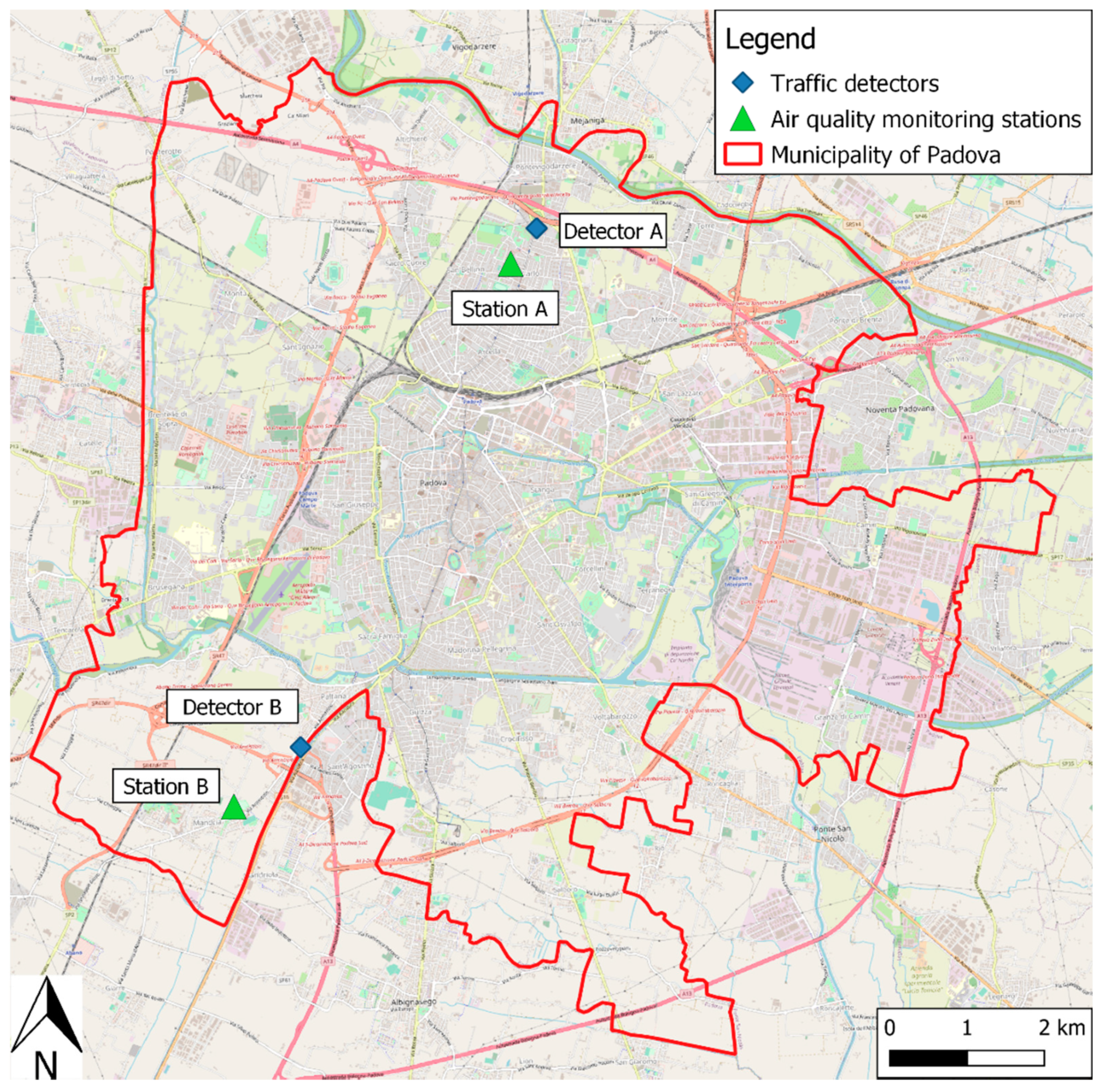
Data on air quality were gathered from two monitoring stations in the study area. Both are located in the urban area of the city (Figure 1): However, Station A is an urban traffic station in the northern part of the city, i.e., recorded pollution levels are mainly affected by emissions from nearby roads [15,40], whereas Station B is an urban background station in the southern part of the city, i.e., recorded pollutant concentrations are not influenced by a single source, but are the integrated contribution from all surrounding sources [15]. The two monitoring sites were selected in order to evaluate and compare the potential relationship between pollutant concentrations and traffic in two sites, thereby testing the strength of the relationship.
Specifically, data were collected by ARPAV, the Veneto Region Environmental Protection Agency, which owns and manages the two stations which record the average daily concentrations of PM10 (in µg/m3) and the hourly concentrations of NO (in µg/m3), NO2 (in µg/m3), and NOx (in µg/m3).
2.3. Traffic Data
Traffic flows were obtained from the automated inductive-loop detectors, managed by the Municipality of Padova and located on road sections along the boundaries of the city. This system collects traffic counts, average speeds, and densities every 10 min, for both inbound and outbound traffic, of four classes of vehicles. The detector closest to each of the two monitoring stations was selected (Figure 1), in order to represent the traffic status in both sites. In detail, Detector A is about 570 m from Station A, and Detector B is about 1170 m from Station B. Data for detector A were available only for outbound traffic; data for detector B were provided for both directions. Since this paper focuses on the effect of reduced traffic on air quality on a city scale, using data obtained both before and during the lockdown due to the COVID-19 pandemic, although the distances between the air quality monitoring stations and traffic detectors were quite high, it is worth noting that the drastic decrease in traffic flows in the lockdown period occurred on a national scale; for this reason, data obtained at a local level may represent the situation on larger scales.
2.4. Meteorological Data
To consider the effect of meteorology on the recorded values of pollutant concentrations, meteorological data were retrieved from the reference site for the province of Padova, managed by ARPAV. The following parameters were recorded on a daily basis, together with minimum and maximum air temperatures (°C), main wind directions and average speeds (m/s), total precipitation (mm), average solar radiation (W/m2), and number of hours with thermal inversion.
2.5. Data Preparation
To analyze the relationship between traffic reduction and air quality, the lockdown period during the COVID-19 pandemic was chosen as a controlled experiment in which traffic flows greatly decreased, thus simulating strict measures on vehicle circulation during normal conditions. For this reason, the days in 2020 when the strictest policies to contain the diffusion of the virus were in force, were compared with the corresponding days in 2017 and 2018 (2019 was not retained, since traffic data were not available for that year). Since PM10 concentrations and meteorological parameters are expressed on a daily basis, the single day was defined as the unit of analysis. Therefore, all the other variables were aggregated; in particular, the average values of NO, NOx, and NO2 concentrations and the total number of vehicles in a day were recorded.
In order to compare days belonging to different years, since this paper is focused on the role of traffic flow, Sundays and holidays (i.e., Easter Sunday Easter Monday and April 25, which is a national holiday in Italy) were discarded, as traffic levels on these days are lower than usual.
As pollutant levels are affected by meteorology, only days with stable meteorological conditions were retained [5,18,25,34,37,40,41,43]. In particular, precipitation level also plays an important role in pollutant concentrations, since it tends to remove particles from the atmosphere [2,5,25,34,39,40]; therefore, only days with no rainfall were considered, thus neglecting the potential confounding effect of this factor. In this way, the final dataset contains only non-rainy days in weekday traffic conditions, in 2020, 2018, and 2017. Thus, the impact of reduced vehicles flows (in 2020) on air quality can be isolated, giving a clear insight into the corresponding potential relationship.
2.6. Relationship between Air Quality and Traffic Levels
To study this relationship, three steps were performed and applied to the values of pollutants recorded by both the monitoring stations.
The first one is to verify whether pollutant concentrations and traffic flows were actually reduced during the lockdown, and to what extent. To reach this aim, a statistical technique was applied to test if the mean values of daily total traffic flows and daily averages of recorded concentrations of NO, NO2, NOx, and PM10 in the considered period of 2020 were lower than the average values on the corresponding days in 2018 and 2017. As data are not normally distributed, a non-parametric Wilcoxon rank-sum test was applied [29].
Then, to evaluate the degree of association between pollutant concentrations, traffic flows, and meteorological parameters, a correlation analysis was developed [5,14,15,30,31,32]. In particular, a non-parametric Spearman’s correlation test was adopted for each day of the period in question.
In order to study the potential effect of traffic flows and meteorology on pollutant concentrations, multivariate linear regression models, which had been widely applied in previous works [5,15,30,32], were implemented. In detail, one model was developed for each daily pollutant concentration (NO, NO2, NOx, PM10) as dependent variables and variable, whereas traffic flows and meteorological parameters considered as independent variables. In addition, in order to follow the assumptions of the model, the natural logarithms of concentrations were used [29]. Other approaches, like machine learning techniques, were not adopted, although they may have produced better accuracy, since the main aim of the paper was to understand the effect of traffic reduction on air quality, and not to predict pollutant concentrations. According to this perspective, a multivariate linear regression model can interpret the effect of each independent factor on the outcome variable, thus clearly analyzing the impact of vehicle flows on pollutant levels.
In descriptive statistics of data and tests on means, data were divided into two periods: The days during the lockdown (in 2020) and the corresponding days before the lockdown (i.e., in 2017 and 2018), for comparison and visualization purposes. Whereas, in the subsequent analyses, each day was individually considered; therefore, a unique dataset made up of all the days in 2020, 2018 and 2017 was adopted.
All analyses were carried out with R statistical software [64].
3. Results
The three-fold statistical analyses were applied in a period from 8 March to 30 April 2020 and to the corresponding days in 2018 and 2017, selecting non-rainy days. In particular, preliminary descriptive statistics were first shown, followed by the results of tests on means and correlation analyses; lastly, the outcomes of multivariate linear regressions are reported. These methods contributed towards creating a clear picture of the effect of traffic flows on all pollutant concentrations (NO, NO2, NOx, PM10).
3.1. Descriptive Statistics
This section presents descriptive statistics of pollutant concentrations and traffic flows for the period in question, in order to provide a preliminary picture of the data distribution (Table 1, Table 2 and Table 3). In particular, Table 1 and Table 2 show descriptive statistics of the sample of concentrations of NO, NO2, NOx, and PM10 recorded by Stations A and B, respectively; in particular, these two tables report the number of observations in the dataset, as well as means, standard deviations, medians, interquartile ranges, and coefficients of variation for the average daily values of considered pollutants. Table 3 shows the corresponding values for total daily traffic flows collected by Detectors A and B. In the following tables, the dataset was split into two groups for comparison purposes: The first set contains days of 2020 and the second one includes days in 2017 and 2018.
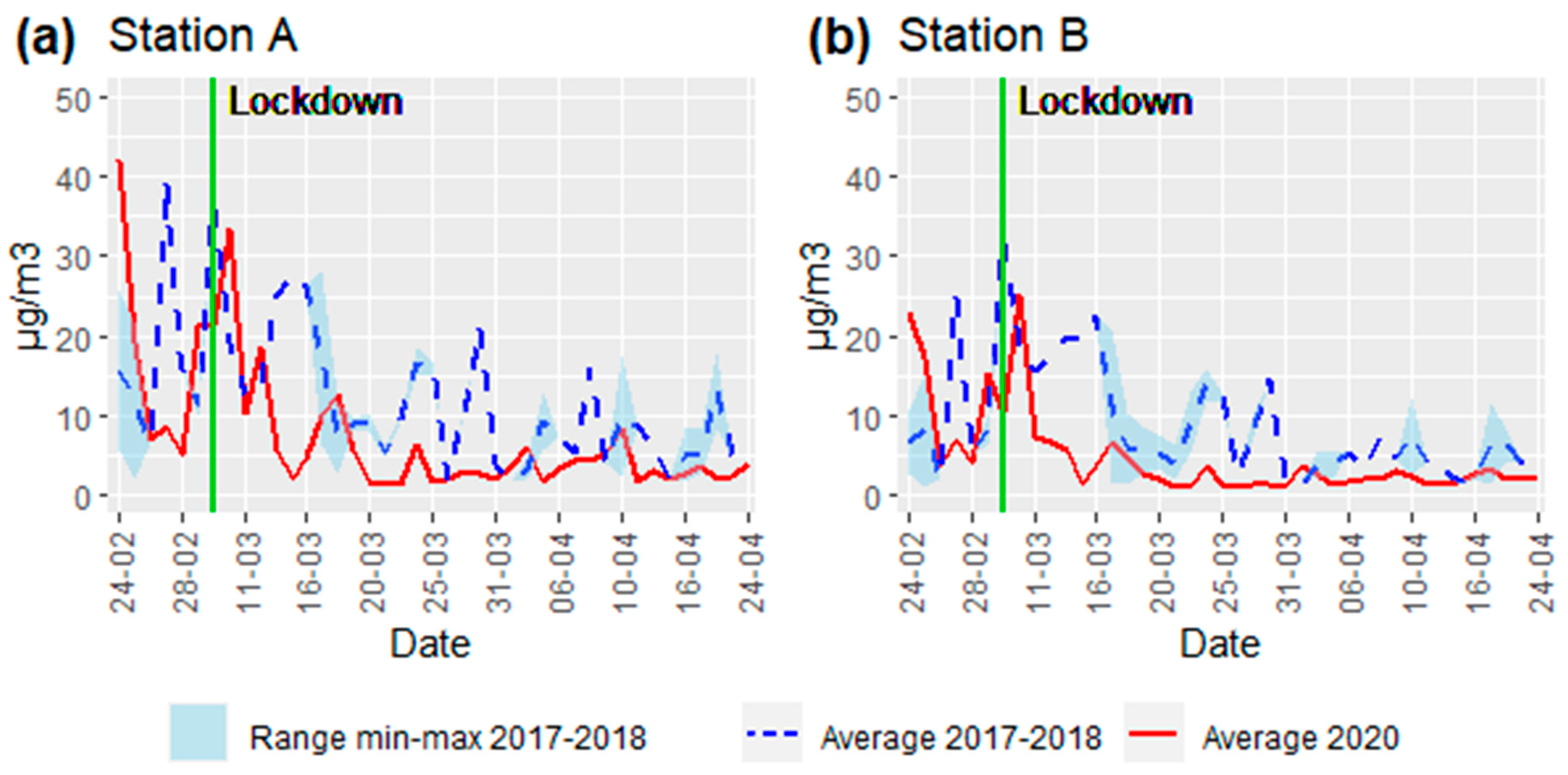
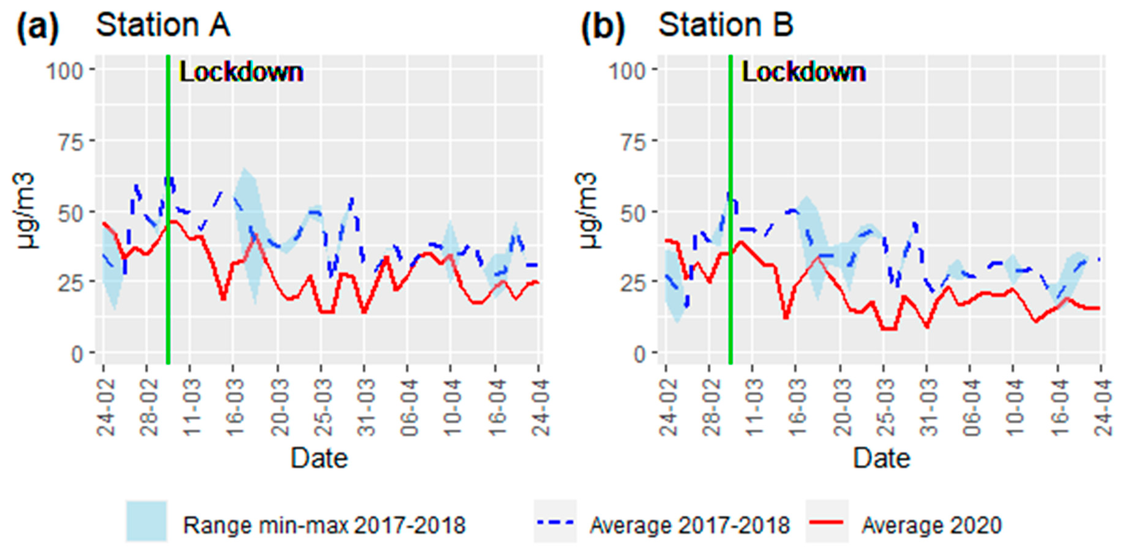
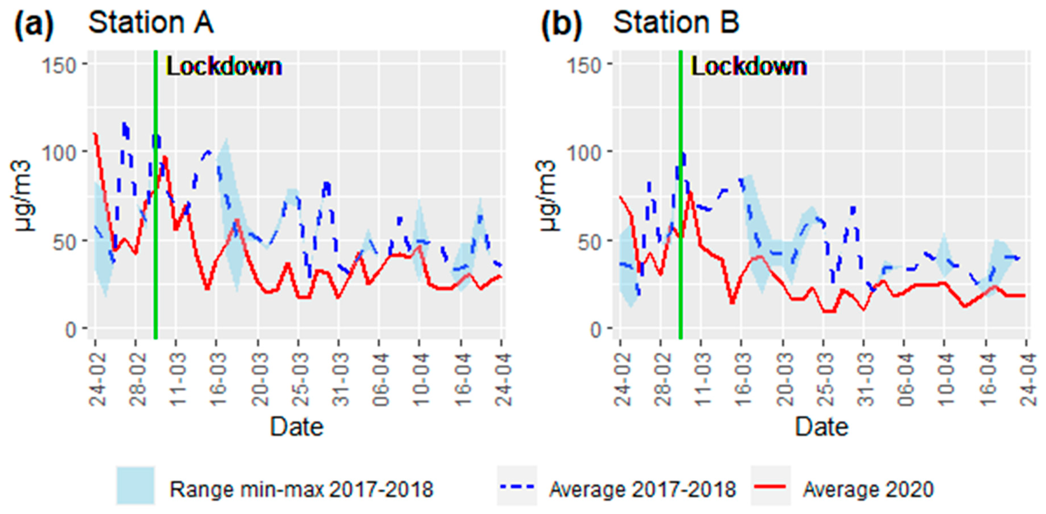
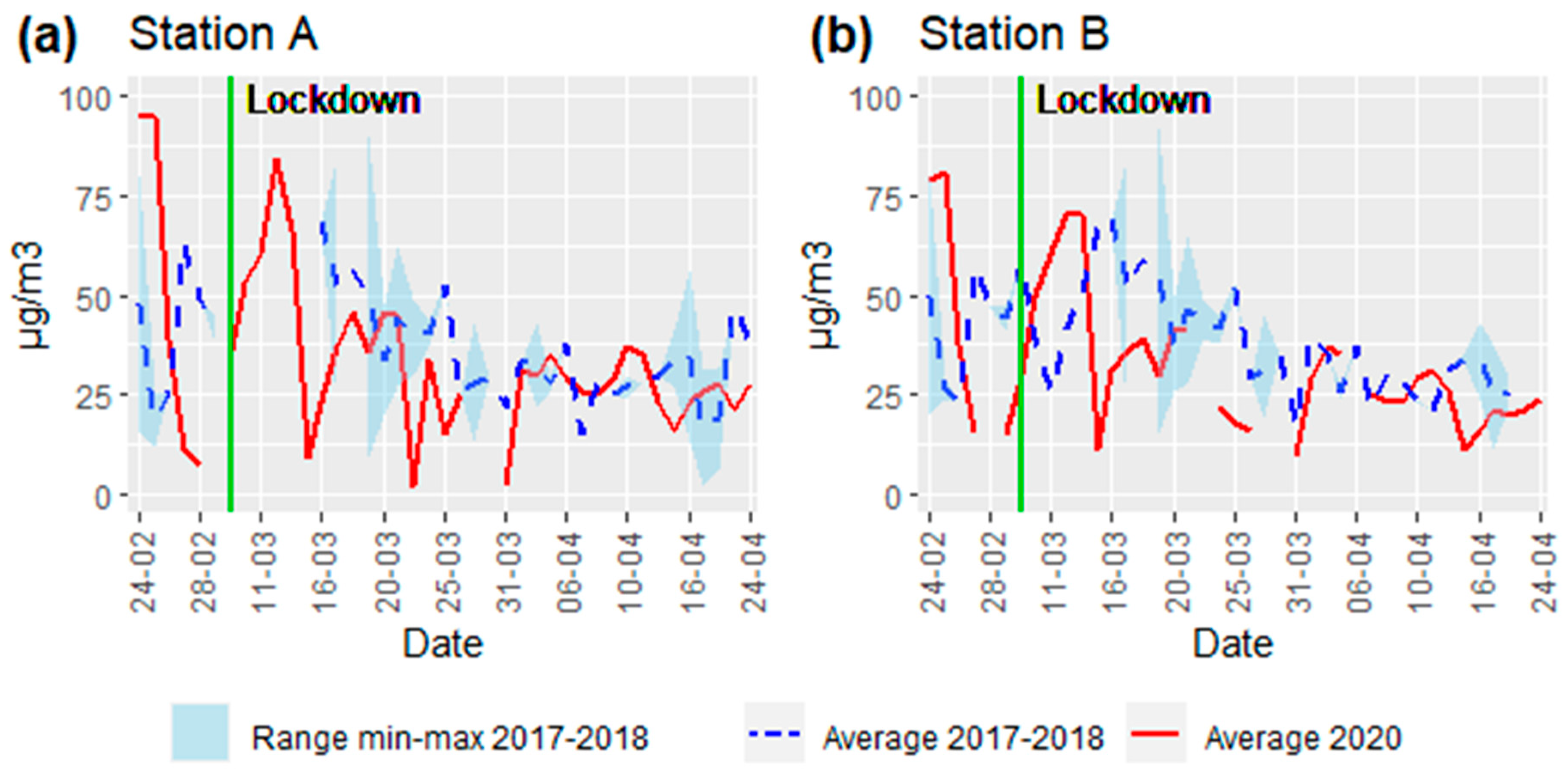
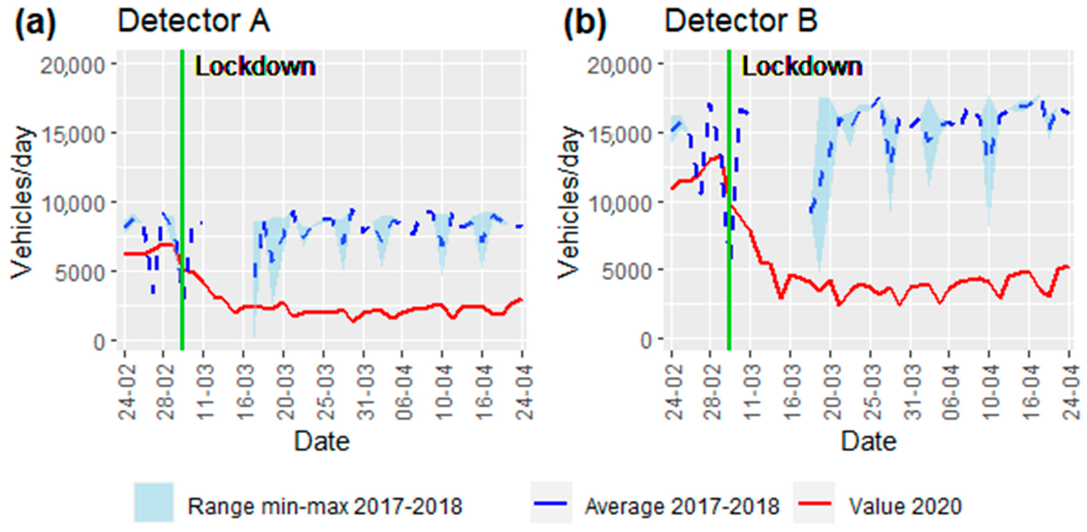
In order to analyze the trends of pollutant concentrations and traffic flows before and during the lockdown due to the COVID-19 pandemic, the following charts were generated extending the period of analysis by a few days before 8 March 2020 (although the following analysis does not consider this extension). Moreover, all the days of the three years were aligned in terms of similar travel habits and mobility needs. Specifically, days were matched according to type of day (e.g., Monday, Tuesday, etc.) and week number in the year. In particular, Figure 2, Figure 3, Figure 4 and Figure 5 show the daily average concentrations of NO (Figure 2), NO2 (Figure 3), NOx (Figure 4), and PM10 (Figure 5) in selected days during 2020, 2018, and 2017, for urban traffic station A and urban background station B). The aim of these figures was to compare the registered values of pollutants in 2020 with those obtained in the same days of 2017 and 2018; for this reason, the horizontal axis indicates the dates in 2020, i.e., each day was matched with the corresponding days of 2018 and 2017. For each day, the solid red line represents the value for 2020, the dashed blue line indicates the average concentration value between days in 2017 and 2018, the pale blue line shows the min-max ranges recorded in 2018 and 2017, and the vertical green line mark the first day of the global lockdown in 2020. Similarly, Figure 6 depicts the total number of vehicles for each day in the selected periods of 2020, 2018, and 2017, for detectors A and B. In this way, values recorded in 2020 were compared with the average and range min-max of values registered in 2017 and 2018. In both figures, lines and colored areas are not all continuous, since some days were excluded because of non-compatible meteorological conditions or public holidays.
Figure 2, Figure 3 and Figure 4 show that, before the lockdown, average concentrations of pollutants were quite similar among the three years. However, after 8 March 2020, the values of NO, NOx, and NO2 for days in 2020 tended to decrease, when compared with the average values of the corresponding days in 2018 and 2017. Instead, PM10 in 2020 does not show a clear-cut reduction with respect to the mean values of 2018 and 2017 (Figure 5). In addition, concentrations for Station A (Figure 2a, Figure 3a, Figure 4a and Figure 5a) are slightly higher than the corresponding values for Station B (Figure 2b, Figure 3b, Figure 4b and Figure 5b). This may be due to the different locations of the two monitoring sites: In fact, with respect to Station B, Station A is closer to the city center, where sources of pollution are more frequent.
Analogously, Figure 6 shows that daily traffic flows significantly fell during the lockdown in 2020, when compared with the average values of the corresponding days in 2018 and 2017. This was an expected result, caused by restrictions to contain the spread of the virus during the COVID-19 lockdown.
3.2. Statistical Comparison between Periods
Table 4 shows the results of the Wilcoxon rank-sum test for all pollutants and monitoring stations. It compares the average values of concentrations recorded during the lockdown (in 2020) with the average value of the corresponding days in 2018 and 2017, in order to assess if the former was lower than the latter. The table shows that significant reductions occurred for NO, NO2, and NOx in both monitoring stations: In particular, in the two periods, NO decreased by 46% (Station A)–54% (Station B), NO2 by 34% (Station A)–40% (Station B), and NOx by 36% (Station A)–44% (Station B). In addition, the corresponding estimated effect sizes are large. Instead, PM10 concentrations were reduced by 2% (Station A)–10% (Station B). However, only the difference calculated for Station B was statistically significant, perhaps due to the different conditions in the two stations.
Table 5 shows the results of the Wilcoxon rank-sum test for daily total traffic flows obtained from the two detectors. The test was applied to verify whether average daily traffic flows in 2020 were lower than average in the corresponding days in 2018 and 2017. Table 4 shows that the mean daily traffic level in 2020 was significantly lower than that for 2018–2017 for both detectors, with a large effect size in both cases. In addition, although Detector A traffic counts were available only for the outbound direction, the percentual reduction (69%) is similar to that obtained from Detector B (71%). This shows that traffic flows consistently decreased in both directions and over a wide area.
The results presented in this section partially confirmed the previous visual analysis. In particular, a comparison of the lockdown days in 2020 with the corresponding days in 2018 and 2017 highlights a statistically significant reduction in traffic flows, and in NO, NO2, and NOx; PM10 significantly decreased for only one station.
3.3. Correlation Analysis
Table 6 shows Spearman’s correlation coefficients and related p-values, which were calculated to evaluate the degree of association among pollutants and traffic flows obtained from detectors at Station A and Station B, and meteorological parameters, for selected non-rainy days. The table shows significant positive correlations between traffic flows and NO, NO2, and NOx; in particular, the highest values of coefficients were obtained for NO2 and NOx. Instead, traffic flows and PM10 are not statistically correlated and show very low coefficients. The results for the two stations are similar, confirming the spatial transferability of results. With regards to meteorological parameters, as expected, correlation coefficients between pollutants and wind speed are negative, since the latter facilitates the dispersion of polluting concentrations in the atmosphere. The relationship with thermal inversion is also significant, since this factor causes unfavorable dispersion of air pollutants emitted at ground levels. In addition, a high significantly negative correlation between pollutant concentration and solar radiation may be observed for PM10. This may be due to the shutdown of heating systems, a source of PM10, because of the relevant contribution of biomass burning for domestic heating in the area [65].
To sum up, the correlation analysis shows that only concentrations of NO, NO2, and NOx are positively associated with traffic flows, confirming results from the previously applied techniques.
3.4. Multivariate Linear Regressions
Results for the multivariate linear regression models are now presented. In particular, Table 7, Table 8, Table 9 and Table 10 show the estimated coefficients, associated statistical tests, and model performances for the daily concentrations of NO (Table 7), NO2 (Table 8), NOx (Table 9), and PM10 (Table 10) from Stations A and B, for selected non-rainy days. Non-significant variables were removed both manually, in order to avoid multicollinearity problems, and an automated stepwise procedure was applied. In all the tables, even non-significant variables were reported using dashes, for better reading and comparing the results of the four regression models.
Table 7, Table 8 and Table 9 show that the coefficients of variables related to traffic flows are all significant and positive, clearly indicating that traffic flows lead to increased concentrations of NO, NO2, and NOx. The same result was obtained at both the monitoring stations, indicating that the effect of traffic on these pollutants extended to most of the whole area. Instead, with regards to the model for PM10 concentrations (Table 10), traffic flows were not identified as significant variables affecting the outcome. This shows that PM10 is not mainly influenced by traffic levels. In addition, the R2 value of these models was lower than the corresponding values in Table 7, Table 8 and Table 9, indicating that other exogenous factors not considered in this model specification may affect PM10 levels.
As regards the effect of meteorological factors in the selected non-rainy days, wind speed negatively affects concentrations of NO, NO2, and NOx, as expected, since it produces a dispersion and dilution of pollutants in the atmosphere [5,25,39,40]. In addition, solar radiation has a negative effect on pollutant levels, as it contributes towards raising the mixing-layer altitude, leading to decreasing concentrations of pollutants in the air [66,67]. Also, the coefficient related to thermal inversions is positive, as expected, since frequent temperature inversions usually affect the formation and suspension of pollutants in the air [68,69]. Lastly, PM10 was found to be positively affected by temperature (Table 10), since it accelerates the chemical process of secondary aerosol formation [32,38], which may surpass the reduced use of heating systems.
4. Discussion and Conclusions
The main aim of this paper was to assess the effectiveness of interventions limiting traffic, such as car-free days or odd-even number-plate schemes, on air quality. Statistical analyses were performed on pollutant concentrations of NO, NO2, NOx, and PM10, traffic counts, and meteorological data collected during the recent lockdown due to the COVID-19 pandemic in Italy, when strict limits were imposed on human activities and transfers in Italy, and also during the corresponding days in 2018 and 2017. In particular, three-fold analysis was applied to selected non-rainy days, in order to control the effect of rain on pollutant concentrations. The approaches were tested on daily air quality data obtained from urban traffic and urban background monitoring stations.
In particular, statistical tests were first applied to evaluate changes in average daily values of traffic flows, NO, NO2, NOx, and PM10 during the lockdown, with respect to the corresponding days in 2018 and 2017. Statistically significant reductions of vehicle flows (by 69–71%), NO (by 46–54%), NO2 (by 34–40%), and NOx (36–44%) were obtained. Conversely, a significant decrease in PM10 was observed at only Station B (10%). The difference between results from the two stations might be due to local characteristics of the areas near the stations. In particular, Station A is set in a residential zone near the city center, whereas Station B is located in a peripherical area, with many different activities as sources of pollutants. In 2015, in Veneto region, 69% of PM10 emissions were generated by combustion of biomass in residential buildings (natural gas is used in most houses to cook and to heat buildings and water), 13% by traffic, 4% by agricultural sector, and 4% by industrial sector [70]. In the same region, no reduction of the use of residential heating systems was registered in March 2020 (lockdown period) with respect to March 2017 [71]. Therefore, unlike Station B, Station A is located in an area where emissions produced by residential activities might not be compensated for the reduction of other PM10 sources, like traffic flows [34,35,42]. The results are consistent with those obtained by previous authors, who reported lowered nitrogen oxide concentrations during the lockdown in many countries [19,24,25,31,37,41,43,44,47,53,57,58,59,60,72]. In addition, the uneven estimated results for PM10 were confirmed by an overall analysis of past researches: Some authors reported reductions in PM10 levels [37,41,43,53] while others did not find any significant changes [24]. Different results were obtained, depending on the considered effect of meteorology and the selected period of analysis [25,29,47,55,56].
Correlation analyses were then carried out, to evaluate the degree of association among pollutant concentrations, traffic flows, and the meteorological factors examined. Results showed that NO, NO2, and NOx were positively correlated with traffic flows. The values of correlation coefficients were consistent with those obtained by previous authors [15,30]. Instead, no significant correlations were found for PM10 and vehicle counts, as in previous works [30]; however, other authors observed low correlation coefficients [5,15].
Multivariate linear regression techniques were then applied to assess the causal relationship between traffic flows and pollutants, with traffic flows and meteorological parameters as independent variables. The results showed that vehicle counts play a significant negative role for concentration levels of NO, NO2, and NOx, as in similar models applied by previous authors [15].
On the other hand, traffic flows did not seem to affect PM10 concentrations to any great extent. As regards the effects of meteorology on the non-rainy days, the impacts of significant factors were consistent with those obtained in other studies; in particular, wind speed has a negative effect [5,25,39,40], as does solar radiation [66,67,73,74,75], whereas thermal inversions positively affect concentrations [45,46,68,69], and PM10 was positively influenced by temperature [32,38,45].
To sum up, all the results of the three approaches are consistent with each other. Specifically, statistical tests on means indicate that, comparing the lockdown period with the corresponding days in 2018 and 2017, despite a significant decrease in traffic flows, PM10 reduction was not statistically significant for one of the two monitoring stations. Moreover, correlation analyses indicated that PM10 concentrations were not correlated with traffic levels, and regression models showed that traffic flows caused changes only in nitrogen oxides. Therefore, the three-fold developed analysis indicates that vehicle flows significantly affect NO, NO2, and NOx concentrations, but there was no evidence of a relationship between traffic and PM10. A similar result was obtained by previous authors [3], who concluded that PM10 levels are not primarily affected by local traffic [2,26,35,42]. The present work confirms these findings, using data recorded during a period in which a drastic and large-scale reduction in traffic flows occurred, thus contributing to strengthening the bases of these conclusions.
According to this perspective, interventions to limit traffic flows, such as car-free days or odd-even number-plate schemes, seem to be effective in improving air quality, but only if the aim of these measures is to reduce NO, NO2, and NOx. Obtained results are helpful in supporting local authorities in optimizing the planning phase of traffic-limitation policies to control air pollution, in order to promote the sustainable development of cities.
Starting from the outcomes of this research, transport policies should be oriented to a global perspective, entailing the changes of travel habits of users towards the use of sustainable transport means. According to this perspective, policies restricting the use of private vehicles should be combined with interventions to foster the adoption of public transport or active modes, such as free public transit tickets to access car-free zones or the design of a wide and safe cycling/pedestrian network. In this way, citizens might experience the possibility to accommodate all their mobility needs, using low-polluting transport modes, thus contributing to the diffusion of long-term sustainable travel habits.
Author Contributions
Conceptualization, R.C., M.G., and R.R.; methodology, R.C., M.G., and R.R.; software, R.C.; validation, M.G. and R.R.; formal analysis, R.C.; data curation, R.C.; writing—original draft preparation, R.C.; writing—review and editing, R.C., M.G., and R.R.; supervision, M.G. and R.R. All authors have read and agreed to the published version of the manuscript.
Funding
This research received no external funding.
Acknowledgments
The authors thank the Municipality of Padova for providing traffic count data, and ARPAV for supporting this work and for providing air quality and meteorological data.
Conflicts of Interest
The authors declare no conflict of interest.
References
- Lähde, T.; Niemi, J.V.; Kousa, A.; Rönkkö, T.; Karjalainen, P.; Keskinen, J.; Frey, A.; Hillamo, R.; Pirjola, L. Mobile Particle and NOx Emission Characterization at Helsinki Downtown: Comparison of Different Traffic Flow Areas. Aerosol Air Qual. Res. 2014, 14, 1372–1382. [Google Scholar] [CrossRef] [Green Version]
- Casale, F.; Nieddu, G.; Burdino, E.; Vignati, D.A.L.; Ferretti, C.; Ugazio, G. Monitoring of submicron particulate matter concentrations in the air of Turin City, Italy. Influence of traffic-limitations. Water Air Soil Pollut. 2009, 196, 141–149. [Google Scholar] [CrossRef]
- Invernizzi, G.; Ruprecht, A.; Mazza, R.; De Marco, C. Measurement of black carbon concentration as an indicator of air quality benefits of traffic restriction policies within the ecopass zone in Milan, Italy. Atmos. Environ. 2011, 45, 3522–3527. [Google Scholar] [CrossRef]
- Madrazo, J.; Clappier, A.; Cuesta, O.; Belalcázar, L.C.; González, Y. Evidence of traffic-generated air pollution in Havana. Atmósfera 2019, 32, 15–24. [Google Scholar] [CrossRef]
- Qu, H.; Lu, X.; Liu, L.; Ye, Y. Environmental Effects of traffic and urban parks on PM10 and PM2.5 mass concentrations. Energy Sources Part A Recovery Util. Environ. Eff. 2019, 1–13. [Google Scholar] [CrossRef]
- Kendrick, C.M.; Koonce, P.; George, L.A. Diurnal and seasonal variations of NO, NO2 and PM2.5 mass as a function of traffic volumes alongside an urban arterial. Atmos. Environ. 2015, 122, 133–141. [Google Scholar] [CrossRef] [Green Version]
- World Health Organization. WHO Air Quality Guidelines for Particulate Matter, Ozone, Nitrogen Dioxide and Sulfur Dioxide; World Health Organization: Geneva, Switzerland, 2005. [Google Scholar]
- ISPRA Infographic on Air Quality and Environment. Available online: https://www.isprambiente.gov.it/files2020/pubblicazioni/stato-ambiente/annuario-2020/Infografiche_r.pdf (accessed on 3 September 2020).
- World Health Organization. Ambient Air Pollution: A Global Assessment of Exposure and Burden of Disease; World Health Organization: Geneva, Switzerland, 2016. [Google Scholar]
- United Nations. The Sustainable Development Goals Report 2020; United Nations: New York, NY, USA, 2020. [Google Scholar]
- European Environment Agency. Air Quality in Europe—2019 Report; European Environment Agency: Copenhagen, Denmark, 2019.
- Baldauf, R.; Watkins, N.; Heist, D.; Bailey, C.; Rowley, P.; Shores, R. Near-road air quality monitoring: Factors affecting network design and interpretation of data. Air Qual. Atmos. Health 2009, 2, 1–9. [Google Scholar] [CrossRef] [Green Version]
- Font, A.; Fuller, G.W. Did policies to abate atmospheric emissions from traffic have a positive effect in London? Environ. Pollut. 2016, 218, 463–474. [Google Scholar] [CrossRef] [Green Version]
- Agudelo-Castañeda, D.M.; Teixeira, E.C.; Rolim, S.B.A.; Pereira, F.N.; Wiegand, F. Measurement of particle number and related pollutant concentrations in an urban area in South Brazil. Atmos. Environ. 2013, 70, 254–262. [Google Scholar] [CrossRef]
- Gualtieri, G.; Crisci, A.; Tartaglia, M.; Toscano, P.; Gioli, B. A Statistical Model to Assess Air Quality Levels at Urban Sites. Wate Air Soil Pollut. 2015, 226, 394. [Google Scholar] [CrossRef]
- Tomassetti, L.; Torre, M.; Tratzi, P.; Paolini, V.; Rizza, V.; Segreto, M.; Petracchini, F.; Tomassetti, L.; Torre, M.; Tratzi, P.; et al. Evaluation of air quality and mobility policies in 14 large Italian cities from 2006 to 2016. J. Environ. Sci. Health Part A 2020, 55, 886–902. [Google Scholar] [CrossRef]
- Pasquier, A.; André, M.; Pasquier, A.; André, M. Considering criteria related to spatial variabilities for the assessment Considering criteria related to spatial variabilities for the assessment of air pollution from traffic of air pollution from traffic. Transp. Res. Procedia 2017, 25, 3354–3369. [Google Scholar] [CrossRef]
- Shi, K.; Di, B.; Zhang, K.; Feng, C.; Svirchev, L. Detrended cross-correlation analysis of urban traffic congestion and NO2 concentrations in Chengdu. Transp. Res. Part D 2018, 61, 165–173. [Google Scholar] [CrossRef]
- Muhammad, S.; Long, X.; Salman, M. COVID-19 pandemic and environmental pollution: A blessing in disguise? Sci. Total Environ. 2020, 728, 138820. [Google Scholar] [CrossRef] [PubMed]
- Kurz, C.; Orthofer, R.; Sturm, P.; Kaiser, A.; Uhrner, U.; Reifeltshammer, R.; Rexeis, M. Urban Climate Projection of the air quality in Vienna between 2005 and 2020 for NO2 and PM10. Urban Clim. 2020, 10, 703–719. [Google Scholar] [CrossRef]
- Cascetta, E. Transportation Systems Analysis: Models and Applications, 2nd ed.; Springer Science & Business Media: Berlin, Germany, 2009; ISBN 978-0-387-75856-5. [Google Scholar]
- United Nations. Resolution adopted by the General Assembly on 25 September 2015; United Nations: New York, NY, USA, 2015. [Google Scholar]
- Perez-martinez, P.J.; Miranda, R.M. Temporal distribution of air quality related to meteorology and road traffic in Madrid. Environ. Monit. Assess. 2015, 187, 220. [Google Scholar] [CrossRef] [PubMed]
- Patel, H.; Talbot, N.; Salmond, J.; Dirks, K.; Xie, S.; Davy, P. Implications for air quality management of changes in air quality during lockdown in Auckland (New Zealand) in response to the 2020 SARS-CoV-2 epidemic. Sci. Total Environ. 2020, 746, 141129. [Google Scholar] [CrossRef] [PubMed]
- Baldasano, J.M. COVID-19 lockdown effects on air quality by NO2 in the cities of Barcelona and Madrid (Spain). Sci. Total Environ. 2020, 741. [Google Scholar] [CrossRef] [PubMed]
- Duque, L.; Relvas, H.; Silveira, C.; Ferreira, J.; Monteiro, A.; Gama, C.; Rafael, S.; Freitas, S.; Borrego, C.; Miranda, A.I. Evaluating strategies to reduce urban air pollution. Atmos. Environ. 2016, 127, 196–204. [Google Scholar] [CrossRef]
- Farda, M.; Balijepalli, C. Exploring the effectiveness of demand management policy in reducing traffic congestion and environmental pollution: Car-free day and odd-even plate measures for Bandung city in Indonesia. Case Stud. Transp. Policy 2018, 6, 577–590. [Google Scholar] [CrossRef]
- Jenkins, N.; Legassick, W.; Sadler, L.; Sokhi, R.S. Correlation Between NO and NO, Roadside Concentrations, Traffic Volumes and Local Meteorology at a Major London Route. WIT Trans. Ecol. Environ. 1995, 6, 405–412. [Google Scholar] [CrossRef]
- Xiang, J.; Austin, E.; Gould, T.; Larson, T.; Shirai, J.; Liu, Y.; Marshall, J.; Seto, E. Impacts of the COVID-19 responses on traffic-related air pollution in a Northwestern US city. Sci. Total Environ. 2020, 747, 141325. [Google Scholar] [CrossRef]
- Roorda-Knape, M.C.; Janssen, N.A.H.; De Hartog, J.J.; Van Vliet, P.H.N.; Harssema, H.; Brunekreef, B. Air pollution from traffic in city disctricts near major motorways. Atmos. Environ. 1998, 32, 1921–1930. [Google Scholar] [CrossRef]
- Wang, Y.; Yuan, Y.; Wang, Q.; Liu, C.; Zhi, Q.; Cao, J. Changes in air quality related to the control of coronavirus in China: Im- plications for traf fi c and industrial emissions. Sci. Total Environ. 2020, 731, 139133. [Google Scholar] [CrossRef]
- Grivas, G.; Chaloulakou, A.; Samara, C.; Spyrellis, N. Spatial and temporal variation of PM10 mass concentrations within the greater area of Athens, Greece. Water Air Soil Pollut. 2004, 2005, 357–371. [Google Scholar] [CrossRef]
- Pan, L.; Yao, E.; Yang, Y. Impact analysis of traffic-related air pollution based on real-time traffic and basic meteorological information. J. Environ. Manag. 2016, 183, 510–520. [Google Scholar] [CrossRef] [PubMed]
- Toscano, D.; Murena, F. The Effect on Air Quality of Lockdown Directives to Prevent the Spread of SARS-CoV-2 Pandemic in Campania Region—Italy: Indications for a Sustainable Development. Sustainability 2020, 12, 5558. [Google Scholar] [CrossRef]
- Menut, L.; Bessagnet, B.; Siour, G.; Mailler, S.; Pennel, R.; Cholakian, A. Impact of lockdown measures to combat Covid-19 on air quality over western Europe. Sci. Total Environ. 2020, 741, 140426. [Google Scholar] [CrossRef] [PubMed]
- Boogaard, H.; Montagne, D.R.; Brandenburg, A.P.; Meliefste, K.; Hoek, G. Comparison of short-term exposure to particle number, PM10 and soot concentrations on three (sub) urban locations. Sci. Total Environ. 2010, 408, 4403–4411. [Google Scholar] [CrossRef] [PubMed]
- Sharma, S.; Zhang, M.; Gao, J.; Zhang, H.; Harsha, S. Effect of restricted emissions during COVID-19 on air quality in India. Sci. Total Environ. 2020, 728, 138878. [Google Scholar] [CrossRef]
- Wang, P.; Chen, K.; Zhu, S.; Wang, P.; Zhang, H. Severe air pollution events not avoided by reduced anthropogenic activities during COVID-19 outbreak. Resour. Conserv. Recycl. 2020, 158, 104814. [Google Scholar] [CrossRef] [PubMed]
- Elminir, H.K. Dependence of urban air pollutants on meteorology. Sci. Total Environ. 2005, 350, 225–237. [Google Scholar] [CrossRef]
- Morelli, X.; Foraster, M.; Aguilera, I.; Basagana, X.; Corradi, E.; Deltell, A. Short-term associations between traffic-related noise, particle number and traffic flow in three European cities. Atmosp. Environ. 2015, 103, 25–33. [Google Scholar] [CrossRef]
- Collivignarelli, M.C.; Abbà, A.; Bertanza, G.; Pedrazzani, R.; Ricciardi, P.; Carnevale Miino, M. Lockdown for CoViD-2019 in Milan: What are the effects on air quality? Sci. Total Environ. 2020, 732, 139280. [Google Scholar] [CrossRef] [PubMed]
- Cameletti, M. The Effect of Corona Virus Lockdown on Air Pollution: Evidence from the City of Brescia in Lombardia Region (Italy). Atmosp. Environ. 2020, 239, 117794. [Google Scholar] [CrossRef]
- Singh, V.; Singh, S.; Biswal, A.; Kesarkar, A.P.; Mor, S. Diurnal and temporal changes in air pollution during COVID-19 strict lockdown over different regions of India*. Environ. Pollut. 2020, 266, 115368. [Google Scholar] [CrossRef]
- Ordóñez, C.; Garrido-perez, J.M.; García-herrera, R. Early spring near-surface ozone in Europe during the COVID-19 shutdown: Meteorological effects outweigh emission changes. Sci. Total Environ. 2020, 747, 141322. [Google Scholar] [CrossRef]
- Olcese, L.E.; Toselli, B.M. Statistical Analysis of PM10 Measurements in Cordoba City, Argentina. Meteorol. Atmos. Phys. 1998, 66, 123–130. [Google Scholar] [CrossRef]
- Trinh, T.T.; Trinh, T.T.; Le, T.T.; Nguyen, T.D.H.; Tu, B.M. Temperature inversion and air pollution relationship, and its effects on human health in Hanoi City, Vietnam. Environ. Geochem. Health 2019, 41, 929–937. [Google Scholar] [CrossRef]
- Tobías, A.; Carnerero, C.; Reche, C.; Massagué, J.; Via, M.; Minguillón, M.C.; Alastuey, A.; Querol, X. Changes in air quality during the lockdown in Barcelona (Spain) one month into the SARS-CoV-2 epidemic. Sci. Total Environ. 2020, 726, 138540. [Google Scholar] [CrossRef]
- Gorbalenya, A.E.; Baker, S.C.; Baric, R.S.; de Groot, R.J.; Drosten, C.; Gulyaeva, A.A.; Haagmans, B.L.; Lauber, C.; Leontovich, A.M.; Neuman, B.W.; et al. The species Severe acute respiratory syndrome-related coronavirus: Classifying 2019-nCoV and naming it SARS-CoV-2. Nat. Microbiol. 2020, 5, 536–544. [Google Scholar] [CrossRef] [Green Version]
- World Health Organization. Coronavirus Disease 2019 (COVID-19) Situation Report–40; World Health Organization: Geneva, Switzerland, 2020. [Google Scholar]
- United Nations United Nations Population Fund-World Population Dashboard. Available online: https://www.unfpa.org/data/world-population-dashboard (accessed on 21 October 2020).
- World Health Organization. Virtual Press Conference on COVID-19–11 March 2020; World Health Organization: Geneva, Switzerland, 2020. [Google Scholar]
- World Health Organization. Coronavirus Disease (COVID-19) Weekly Epidemiological Update; World Health Organization: Geneva, Switzerland, 2020. [Google Scholar]
- Dantas, G.; Siciliano, B.; França, B.B.; da Silva, C.M.; Arbilla, G. The impact of COVID-19 partial lockdown on the air quality of the city of Rio de Janeiro, Brazil. Sci. Total Environ. 2020, 729, 139085. [Google Scholar] [CrossRef] [PubMed]
- Kumar, P.; Hama, S.; Omidvarborna, H.; Sharma, A.; Sahani, J.; Abhijith, K.V.; Debele, S.E.; Zavala-reyes, J.C.; Barwise, Y.; Tiwari, A. Temporary reduction in fine particulate matter due to ‘anthropogenic emissions switch-off’ during COVID-19 lockdown in Indian cities. Sustain. Cities Soc. 2020, 62, 102382. [Google Scholar] [CrossRef] [PubMed]
- Zangari, S.; Hill, D.T.; Charette, A.T.; Mirowsky, J.E. Air quality changes in New York City during the COVID-19 pandemic. Sci. Total Environ. 2020, 742, 140496. [Google Scholar] [CrossRef]
- Jia, C.; Fu, X.; Bartelli, D.; Smith, L. Insignificant Impact of the “Stay-At-Home” Order on Ambient Air Quality in the Memphis Metropolitan Area, U.S.A. Atmosphere 2020, 11, 630. [Google Scholar] [CrossRef]
- Lian, X.; Huang, J.; Huang, R.; Liu, C.; Wang, L.; Zhang, T. Impact of city lockdown on the air quality of COVID-19-hit of Wuhan city. Sci. Total Environ. 2020, 742, 140556. [Google Scholar] [CrossRef]
- Aloi, A.; Alonso, B.; Benavente, J.; Cordera, R.; Echániz, E.; González, F.; Ladisa, C.; Lezama-Romanelli, R.; López-Parra, Á.; Mazzei, V.; et al. Effects of the COVID-19 lockdown on urban mobility: Empirical evidence from the city of Santander (Spain). Sustainability 2020, 12, 3870. [Google Scholar] [CrossRef]
- Connerton, P.; de Assunção, J.V.; de Miranda, R.M.; Slovic, A.D.; Pérez-Martínez, P.J.; Ribeiro, H. Air quality during covid-19 in four megacities: Lessons and challenges for public health. Int. J. Environ. Res. Public Health 2020, 17, 5067. [Google Scholar] [CrossRef]
- Yuri, L.; Nakada, K.; Custodio, R. COVID-19 pandemic: Impacts on the air quality during the partial lockdown in São Paulo state, Brazil. Sci. Total Environ. 2020, 730, 139087. [Google Scholar] [CrossRef]
- Comune di Padova. Annuario Statistico Comunale-Capitolo 2; Comune di Padova: Padova, Italy, 2019. [Google Scholar]
- Comune di Padova. Annuario Statistico Comunale-Capitolo 1; Comune di Padova: Padova, Italy, 2018. [Google Scholar]
- Agenzia Regionale per la Prevenzione e protezione Ambientale del Veneto (ARPAV). Air Quality in the Veneto Region.-Annual Report; Agenzia Regionale per la Prevenzione e protezione Ambientale del Veneto (ARPAV): Padova, Italy, 2019. [Google Scholar]
- European Environmental Agency. R Core Team. R: A Language and Environment for Statistical Computing; European Environmental Agency: Copenhagen, Denmark, 2019.
- Patti, S.; Pillon, S.; Intini, B.; Susanetti, L. PREPAIR-Po Regions Engaged to Policies of AIR. Action D3: Residential Wood Consumption Estimation in the Po Valley-Report on the Survey to Estimate Woody Biomasses Consumption in Households. 2020. Available online: http://www.lifeprepair.eu/wp-content/uploads/2017/06/D3_Report-on-woody-biomasses-consumption-in-households_01feb2020-1.pdf (accessed on 21 October 2020).
- Tie, X.; Huang, R.J.; Cao, J.; Zhang, Q.; Cheng, Y.; Su, H.; Chang, D.; Pöschl, U.; Hoffmann, T.; Dusek, U.; et al. Severe Pollution in China Amplified by Atmospheric Moisture. Sci. Rep. 2017, 7, 1–8. [Google Scholar] [CrossRef]
- Feng, X.; Wu, B.; Yan, N. A method for deriving the boundary layer mixing height from MODIS atmospheric profile data. Atmosphere 2015, 6, 1346–1361. [Google Scholar] [CrossRef] [Green Version]
- Masiol, M.; Squizzato, S.; Formenton, G.; Harrison, R.M.; Agostinelli, C. Air quality across a European hotspot: Spatial gradients, seasonality, diurnal cycles and trends in the Veneto region, NE Italy. Sci. Total Environ. 2017, 576, 210–224. [Google Scholar] [CrossRef]
- Malek, E.; Davis, T.; Martin, R.S.; Silva, P.J. Meteorological and environmental aspects of one of the worst national air pollution episodes (January, 2004) in Logan, Cache Valley, Utah, USA. Atmos. Res. 2006, 79, 108–122. [Google Scholar] [CrossRef]
- Agenzia Regionale per la Prevenzione e protezione Ambientale del Veneto (ARPAV). Inventario Regionale Delle Emissioni in Atmosfera Inemar Veneto 2015-Risultati Dell’edizione 2015-Relazione Generale. 2019. Available online: https://www.arpa.veneto.it/temi-ambientali/aria/file-e-allegati/relazione-inemar-2015/RELAZIONE%20GENERALE%20-%20INEMAR%20Veneto%202015.pdf (accessed on 21 October 2020).
- Agenzia Regionale per la Prevenzione e protezione Ambientale del Veneto (ARPAV). Effetti Del Lockdown Durante L’ Emergenza COVID-19 in Veneto. 2020. Available online: https://www.snpambiente.it/2020/05/25/effetti-del-lockdown-durante-lemergenza-covid-19-in-veneto/ (accessed on 21 October 2020).
- Wang, Q.; Su, M. A preliminary assessment of the impact of COVID-19 on environment—A case study of China. Sci. Total Environ. 2020, 728, 138915. [Google Scholar] [CrossRef]
- Ulke, A.G.; Mazzeo, N.A. Climatological aspects of the daytime mixing height in Buenos Aires city, Argentina. Atmosp. Environ. 1998, 32, 1615–1622. [Google Scholar] [CrossRef]
- Mazzeo, N.A.; Venegas, L.E.; Choren, H. Analysis of NO, NO2, O3 and NOx concentrations measured at a green area of Buenos Aires City during wintertime. Atmosp. Environ. 2005, 39, 3055–3068. [Google Scholar] [CrossRef]
- Han, S.; Bian, H.; Feng, Y.; Liu, A.; Li, X.; Zeng, F.; Zhang, X. Analysis of the relationship between O3, NO and NO2 in Tianjin, China. Aerosol. Air Qual. Res. 2011, 11, 128–139. [Google Scholar] [CrossRef] [Green Version]
Figure 1.
Study area and locations of traffic detectors and air quality monitoring stations.

Figure 2.
Average daily concentrations of NO for selected days in 2020, 2018, and 2017, for (a) Station A and (b) Station B.
Figure 2.
Average daily concentrations of NO for selected days in 2020, 2018, and 2017, for (a) Station A and (b) Station B.

Figure 3.
Average daily concentrations of NO2 for selected days in 2020, 2018, and 2017, for (a) Station A and (b) Station B.
Figure 3.
Average daily concentrations of NO2 for selected days in 2020, 2018, and 2017, for (a) Station A and (b) Station B.

Figure 4.
Average daily concentrations of NOx for selected days in 2020, 2018, and 2017, for (a) Station A and (b) Station B.
Figure 4.
Average daily concentrations of NOx for selected days in 2020, 2018, and 2017, for (a) Station A and (b) Station B.

Figure 5.
Average daily concentrations of PM10 for selected days in 2020, 2018, and 2017, for (a) Station A and (b) Station B.
Figure 5.
Average daily concentrations of PM10 for selected days in 2020, 2018, and 2017, for (a) Station A and (b) Station B.

Figure 6.
Total number of vehicles per day in 2020, 2018, and 2017 for selected days in 2020, 2018 and 2017, for detectors (a) A and (b) B.
Figure 6.
Total number of vehicles per day in 2020, 2018, and 2017 for selected days in 2020, 2018 and 2017, for detectors (a) A and (b) B.


Table 1.
Descriptive statistics for concentrations of NO, NO2, NOx, and PM10 for Station A.
| NO | NO2 | NOx | PM10 | |||||
|---|---|---|---|---|---|---|---|---|
| 2017–2018 | 2020 | 2017–2018 | 2020 | 2017–2018 | 2020 | 2017–2018 | 2020 | |
| N. of observations | 56 | 38 | 54 | 40 | 55 | 39 | 57 | 35 |
| Mean [μg/m3] | 10.04 | 5.41 | 39.67 | 26.06 | 54.21 | 34.52 | 36.07 | 35.40 |
| Std. Dev. 1 [μg/m3] | 7.13 | 6.52 | 8.99 | 9.09 | 19.93 | 18.04 | 16.92 | 18.84 |
| Median [μg/m3] | 7.94 | 3.02 | 38.30 | 24.10 | 49.69 | 29.90 | 32.50 | 30.00 |
| IQR 2 [μg/m3] | 9.58 | 3.73 | 13.04 | 13.52 | 27.26 | 18.81 | 18.50 | 12.00 |
| CV 3 | 71 | 121 | 23 | 35 | 37 | 52 | 47 | 54 |
1 Standard deviation; 2 Interquartile range; 3 Coefficient of variation.
Table 2.
Descriptive statistics for concentrations of NO, NO2, NOx, and PM10 for Station B.
| NO | NO2 | NOx | PM10 | |||||
|---|---|---|---|---|---|---|---|---|
| 2017–2018 | 2020 | 2017–2018 | 2020 | 2017–2018 | 2020 | 2017–2018 | 2020 | |
| N. of observations | 53 | 39 | 53 | 39 | 53 | 39 | 57 | 35 |
| Mean [μg/m3] | 6.92 | 3.15 | 32.23 | 19.46 | 42.54 | 24.00 | 36.56 | 32.85 |
| Std. Dev. 1 [μg/m3] | 4.95 | 4.19 | 8.36 | 7.91 | 15.36 | 13.53 | 15.71 | 18.69 |
| Median [μg/m3] | 5.13 | 1.82 | 31.10 | 17.60 | 39.21 | 19.09 | 35.00 | 27.50 |
| IQR 2 [μg/m3] | 6.79 | 2.15 | 11.27 | 8.19 | 18.04 | 10.26 | 16.00 | 15.50 |
| CV 3 | 72 | 132 | 26 | 41 | 36 | 56 | 43 | 57 |
1 Standard deviation; 2 Interquartile range; 3 Coefficient of variation.
Table 3.
Descriptive statistics for traffic flows recorded by two detectors.
| Detector A | Detector B | |||
|---|---|---|---|---|
| 2017–2018 | 2020 | 2017–2018 | 2020 | |
| N. of observations | 56 | 38 | 53 | 39 |
| Mean [veh/day] | 7605 | 2341 | 14,650 | 4182 |
| Std. Dev. 1 [veh/day] | 1916 | 904 | 3394 | 1682 |
| Median [veh/day] | 8354 | 2228 | 15,930 | 4036 |
| IQR 2 [veh/day] | 1372 | 549 | 2300 | 1234 |
| CV 3 | 25 | 39 | 23 | 40 |
1 Standard deviation; 2 Interquartile range; 3 Coefficient of variation.
Table 4.
Results of Wilcoxon rank-sum test and effect size calculations for comparison of daily average values of pollutant concentrations [μg/m3] between 2020 and 2018–2017 for two monitoring stations.
Table 4.
Results of Wilcoxon rank-sum test and effect size calculations for comparison of daily average values of pollutant concentrations [μg/m3] between 2020 and 2018–2017 for two monitoring stations.
| Station A | Station B | |||||||||
|---|---|---|---|---|---|---|---|---|---|---|
| Variable | Avg. 2018–2017 | Avg. 2020 | W-Test | p-Value | Effect Size | Avg. 2018–2017 | Avg. 2020 | W-Test | p-Value | Effect Size |
| NO | 10.04 | 5.41 | 501 | 0.000 | 0.45 | 6.920 | 3.150 | 391 | 0.000 | 0.53 |
| NO2 | 39.67 | 26.06 | 314 | 0.000 | 0.61 | 32.230 | 19.460 | 283 | 0.000 | 0.62 |
| NOx | 54.21 | 34.52 | 427 | 0.000 | 0.51 | 42.540 | 24.000 | 308 | 0.000 | 0.60 |
| PM10 | 36.07 | 35.40 | 875 | 0.200 | 0.09 | 36.560 | 32.850 | 725 | 0.020 | 0.21 |
Table 5.
Results of Wilcoxon rank-sum test and effect size calculations for comparison of daily total vehicle flows [veh/day] between 2020 and 2018-2017 for two traffic flow detectors.
Table 5.
Results of Wilcoxon rank-sum test and effect size calculations for comparison of daily total vehicle flows [veh/day] between 2020 and 2018-2017 for two traffic flow detectors.
| Detector A | Detector B | |||||||||
|---|---|---|---|---|---|---|---|---|---|---|
| Variable | Avg. 2018–2017 | Avg. 2020 | W-Test | p-Value | Effect Size | Avg. 2018–2017 | Avg. 2020 | W-Test | p-Value | Effect Size |
| Traffic flow | 7605 | 2341 | 58 | 0.000 | 0.80 | 14,650 | 4182 | 28 | 0.000 | 0.83 |
Table 6.
Spearman’s correlation coefficients and p-values among traffic flows, pollutant concentrations, and meteorological parameters for two monitoring stations.
Table 6.
Spearman’s correlation coefficients and p-values among traffic flows, pollutant concentrations, and meteorological parameters for two monitoring stations.
| Station A | Station B | |||||||
|---|---|---|---|---|---|---|---|---|
| NO | NO2 | NOx | PM10 | NO | NO2 | NOx | PM10 | |
| Traffic flow | +0.51 *** | +0.56 *** | +0.55 *** | +0.14 | +0.63 *** | +0.66 *** | +0.66 *** | +0.16 |
| Minimum temperature | −0.18 | −0.09 | −0.14 | +0.08 | −0.12 | +0.08 | +0.02 | −0.01 |
| Maximum temperature | +0.06 | +0.08 | +0.06 | −0.01 | +0.09 | +0.16 | +0.14 | −0.07 |
| Solar radiation | −0.21 † | −0.22 † | −0.22 † | −0.55 *** | −0.12 | −0.22 † | −0.20 † | −0.53 *** |
| Thermal inversion | +0.44 *** | +0.40 *** | +0.43 *** | +0.14 | +0.41 *** | +0.36 ** | +0.37 *** | +0.16 |
| Wind speed | −0.47 *** | −0.41 *** | −0.44 *** | −0.39 *** | −0.48 *** | −0.44 *** | −0.45 *** | −0.40 *** |
Significance codes for p-value of correlation: *** p-value ≤ 0.001; ** p-value ≤ 0.01; * p-value ≤ 0.05; † p-value ≤ 0.10.
Table 7.
Multivariate linear regression for NO concentrations.
| Station A | Station B | |||||||
|---|---|---|---|---|---|---|---|---|
| Variable | Coeff. | Std. Err. | t-Value | p-Value | Coeff. | Std. Err. | t-Value | p-Value |
| Intercept | 0.774 | 0.138 | 5.60 | 0.000 *** | 0.470 | 0.116 | 4.05 | 0.000 *** |
| Traffic flow | 0.067 | 0.008 | 8.31 | 0.000 *** | 0.040 | 0.004 | 10.00 | 0.000 *** |
| Wind speed | −0.067 | 0.027 | −2.50 | 0.014 * | −0.074 | 0.026 | −2.85 | 0.006 ** |
| Solar radiation | −0.003 | 0.000 | −6.00 | 0.000 *** | −0.003 | 0.000 | −6.67 | 0.000 *** |
| Thermal inversion | 0.052 | 0.007 | 7.49 | 0.000 *** | 0.043 | 0.007 | 6.34 | 0.000 *** |
| Maximum temperature | – | – | – | – | – | – | – | – |
| Statistics | ||||||||
| N | 94 | 92 | ||||||
| Adj. R2 | 0.65 | 0.68 | ||||||
| F-stat | 35.95 | p-value | 0.000 *** | 50.22 | p-value | 0.000 *** | ||
Significance codes for p-value: *** p-value ≤ 0.001; ** p-value ≤ 0.01; * p-value ≤ 0.05; † p-value ≤ 0.10.
Table 8.
Multivariate linear regression for NO2 concentrations.
| Station A | Station B | |||||||
|---|---|---|---|---|---|---|---|---|
| Variable | Coeff. | Std. Err. | t-Value | p-Value | Coeff. | Std. Err. | t-Value | p-Value |
| Intercept | 1.377 | 0.048 | 28.79 | 0.000 *** | 1.363 | 0.047 | 28.82 | 0.000 *** |
| Traffic flow | 0.034 | 0.003 | 10.39 | 0.000 *** | 0.022 | 0.002 | 13.43 | 0.000 *** |
| Wind speed | −0.019 | 0.010 | −1.98 | 0.050 * | −0.036 | 0.011 | −3.29 | 0.001 ** |
| Solar radiation | −0.001 | 0.000 | −5.16 | 0.000 *** | −0.001 | 0.000 | −7.78 | 0.000 *** |
| Thermal inversion | 0.018 | 0.003 | 6.33 | 0.000 *** | 0.017 | 0.003 | 5.82 | 0.000 *** |
| Maximum temperature | – | – | – | – | – | – | – | – |
| Statistics | ||||||||
| N | 94 | 92 | ||||||
| Adj. R2 | 0.68 | 0.77 | ||||||
| F–stat | 49.53 | p-value | 0.000 *** | 75.24 | p-value | 0.000 *** | ||
Significance codes for p-value: *** p-value ≤ 0.001; ** p-value ≤ 0.01; * p-value ≤ 0.05; † p-value ≤ 0.10.
Table 9.
Multivariate linear regression for NOx concentrations.
| Station A | Station B | |||||||
|---|---|---|---|---|---|---|---|---|
| Variable | Coeff. | Std. Err. | t-Value | p-Value | Coeff. | Std. Err. | t-Value | p-Value |
| Intercept | 1.499 | 0.065 | 23.18 | 0.000 *** | 1.416 | 0.055 | 25.81 | 0.000 *** |
| Traffic flow | 0.041 | 0.004 | 9.53 | 0.000 *** | 0.027 | 0.002 | 14.13 | 0.000 *** |
| Wind speed | −0.027 | 0.014 | −1.89 | 0.063 † | −0.041 | 0.011 | −3.60 | 0.001 *** |
| Solar radiation | −0.001 | 0.000 | −6.59 | 0.000 *** | −0.002 | 0.000 | −8.12 | 0.000 *** |
| Thermal inversion | 0.028 | 0.004 | 7.61 | 0.000 *** | 0.022 | 0.003 | 6.64 | 0.000 *** |
| Maximum temperature | – | – | – | – | – | – | – | – |
| Statistics | ||||||||
| N | 94 | 92 | ||||||
| Adj. R2 | 0.67 | 0.79 | ||||||
| F–stat | 47.15 | p-value | 0.000 *** | 87.26 | p-value | 0.000 *** | ||
Significance codes for p-value: *** p-value ≤ 0.001; ** p-value ≤ 0.01; * p-value ≤ 0.05; † p-value ≤ 0.10.
Table 10.
Multivariate linear regression for PM10 concentrations.
| Station A | Station B | |||||||
|---|---|---|---|---|---|---|---|---|
| Variable | Coeff. | Std. Err. | t-Value | p-Value | Coeff. | Std. Err. | t-Value | p-Value |
| Intercept | 1.725 | 0.074 | 23.32 | 0.000 *** | 1.786 | 0.066 | 27.22 | 0.000 *** |
| Traffic flow | – | – | – | – | – | – | – | – |
| Wind speed | – | – | – | – | – | – | – | – |
| Solar radiation | −0.003 | 0.000 | −9.45 | 0.000 *** | −0.003 | 0.000 | −10.11 | 0.000 *** |
| Thermal inversion | 0.015 | 0.004 | 3.75 | 0.000 *** | 0.010 | 0.003 | 2.99 | 0.004 ** |
| Maximum temperature | 0.017 | 0.004 | 3.97 | 0.000 *** | 0.013 | 0.004 | 3.50 | 0.001 *** |
| Statistics | ||||||||
| N | 94 | 92 | ||||||
| Adj. R2 | 0.50 | 0.53 | ||||||
| F–stat | 30.62 | p-value | 0.000 *** | 34.83 | p-value | 0.000 *** | ||
Significance codes for p-value: *** p-value ≤ 0.001; ** p-value ≤ 0.01; * p-value ≤ 0.05; † p-value ≤ 0.10.
Publisher’s Note: MDPI stays neutral with regard to jurisdictional claims in published maps and institutional affiliations. |
© 2020 by the authors. Licensee MDPI, Basel, Switzerland. This article is an open access article distributed under the terms and conditions of the Creative Commons Attribution (CC BY) license (http://creativecommons.org/licenses/by/4.0/).
Share and Cite
MDPI and ACS Style
Rossi, R.; Ceccato, R.; Gastaldi, M. Effect of Road Traffic on Air Pollution. Experimental Evidence from COVID-19 Lockdown. Sustainability 2020, 12, 8984. https://doi.org/10.3390/su12218984
AMA Style
Rossi R, Ceccato R, Gastaldi M. Effect of Road Traffic on Air Pollution. Experimental Evidence from COVID-19 Lockdown. Sustainability. 2020; 12(21):8984. https://doi.org/10.3390/su12218984
Chicago/Turabian StyleRossi, Riccardo, Riccardo Ceccato, and Massimiliano Gastaldi. 2020. "Effect of Road Traffic on Air Pollution. Experimental Evidence from COVID-19 Lockdown" Sustainability 12, no. 21: 8984. https://doi.org/10.3390/su12218984
Note that from the first issue of 2016, this journal uses article numbers instead of page numbers. See further details here.