
Analysis of the Impact of the COVID-19 Pandemic on the Value of CO2 Emissions from Electricity Generation


Faculty of Security, Logistics and Management, Military University of Technology, 00-908 Warsaw, Poland
*
Author to whom correspondence should be addressed.
Energies 2022, 15(13), 4514; https://doi.org/10.3390/en15134514
Submission received: 30 May 2022
/
Revised: 17 June 2022
/
Accepted: 19 June 2022
/
Published: 21 June 2022
(This article belongs to the Special Issue Energy Consumption in EU Countries)
Abstract
:The study analyzed the impact of the COVID-19 pandemic on the carbon dioxide emissions from electricity generation. Additionally, monthly seasonality was taken into account. It was assumed (research hypothesis) that both the COVID-19 pandemic (expressed in individual waves of infection cases) and the month have a significant impact on CO2 emissions. Analysis of variance (ANOVA) and non-parametric Kruskal–Wallis tests were used to evaluate the significance of the influence of individual explanatory variables on the CO2 emission. The identification of the studied series (CO2 emission) was first made by means of a linear regression model with binary variables and then by the ARMAX model. The analysis shows that in the consecutive months and periods of the COVID-19 pandemic, CO2 emissions differ significantly. The highest increase in emissions was recorded for the second wave of the pandemic, as well as in January and February. This is due to the overlapping of both the increase in infections (favoring stays at home) and the winter season. It can be concluded that working plants, schools and factories had the same demand for electricity, but sources of increased consumption were people staying at home and in hospitals as a result of deteriorated health, isolation or quarantine.
1. Introduction
Carbon dioxide is an inorganic colorless gas heavier than air. It exists in trace amounts in the atmosphere, but it has a huge impact on the greenhouse effect, which is harmful to Earth [1,2]. Greenhouse gases become trapped in the atmosphere, forming a layer that impedes the transfer of heat from Earth’s interior to space, consequently causing the planet’s temperature to rise [3]. In Poland, which is the subject of this study, the dominant source of electricity generation is still both lignite and hard coal [4]. Coal-fired power plants provide about 70% of the installed capacity; they are characterized by low flexibility, i.e., the ability to respond quickly to fluctuations in power demand under conditions of high energy consumption [5]. Unfortunately, the production of electricity from this source results in high emissions of environmentally harmful carbon dioxide, so it is an important subject of research. There are various factors influencing electricity generation, including time of day, season and, as observations have shown, also emergency events. An example of such a situation is a state of pandemic. In Poland, the pandemic started in March 2020. The new coronavirus pandemic initially paralyzed the world. The negative impact of lockdown and other restrictions has been reported for the economy [6,7], tourism [8], culture [9], sporting events [10,11], education [12,13] and politics [14,15]. Such a large impact of the COVID-19 pandemic on various economic or social areas is also generating interest in its impact on the energy and environmental areas, as evidenced by numerous scientific publications appearing in this area. The environmental sector is directly related to energy, which is a part of the economy that should be very flexible as it is affected by many factors, such as time of day, time of year, stock market fluctuations, politics, CO2 allowance prices and many others. Crisis situations, such as pandemics, also test its flexibility and variability. This is discussed, among others, by M. Kędzierski et al., who in their paper [5] focus on analyzing the relationship between relaxing and tightening restrictions using the “transformation curve”. The authors analyzed the correlation between reproduction rate (a rate that tells how many people one sick person can infect) and energy demand and mobility (related to the restriction index) by comparing data for 18 European countries for the period 1 April–27 July 2020. The article mainly focuses on electricity generation itself and does not address environmental issues.
H. L. Gabryś in his paper [16] links the dependence of electricity generation to the extraction (consumption) of both lignite and hard coal in the first period of the pandemic and the period before its onset. The author shows a clear decline in coal mining efficiency during the pandemic period. In [17], Vinicius B.F. et al. analyzed, using stochastic simulation, the impact of the pandemic on the electricity market from a socio-economic perspective and a forecast for the post-pandemic period. The research focused on countries such as Germany, USA, China, India and Italy. The authors proposed a stochastic socio-economic model of a time series to analyze the impact of the pandemic on the electricity market. The method described combining an optimized tariff model (a socioeconomic market model) and the concept of random straying (a risk assessment technique). The purpose of the model is to identify past events and forecast future ones. Ultimately, the authors suggest the validity of using other tools, including models such as ARIMA, Holt–Winter or artificial intelligence. On the other hand, in [18], Ahmad M. and other authors used a mathematical model to evaluate the effects of the pandemic and curfew on average hourly electrical load. The following conclusions were drawn from the analysis: electricity generation decreased to about 16.4% compared to the previous year; electrical load varied depending on the time of year; and curfew enforcement was associated with a further decrease in generation to 16.4%, but only between 12:00 and 6:00 pm. In addition, a within-sector analysis could examine whether policymakers can use electricity load data as a real-time indicator of factors such as the impact of the pandemic on economic activity (e.g., a decline in commercial electricity demand due to a recession) or people’s compliance with movement restriction orders (e.g., whether people are complying with stay-at-home orders). Future research may also evaluate the impact of COVID-19 mitigation measures on other important issues, e.g., fuel supply chain, environment, economy, etc., in different contexts and settings (e.g., other regions with different climate and energy subsidy structures).
On the other hand, E. Yukseltan et al. in their paper [19] made predictions regarding the impact of constraints on total electricity demand in Turkey using modular Fourier series expansion. This paper analyzes the impact of unexpected factors, in this case the COVID-19 pandemic, on electricity generation. To analyze the impact of the pandemic on the demand and daily electricity profile, Fourier transform was used to evaluate deviations from normal conditions. Studies show a marked decrease in electricity consumption during the first phase of the pandemic. The authors also analyzed the shape of the daily demand curve to present how demand shifted from daytime to nighttime. A population-based constraint index was proposed to analyze the relationship between the strength and extent of constraints and total demand. The analyses conducted suggest that new approaches to scheduling daily and weekly loads are needed to avoid future mismatches between supply and demand.
In [20], Stephanie Halbrügge et al. performed an analysis on grid frequency and balancing power. In particular, electricity transmission in Germany was considered. The need to analyze the possibility of expanding the flexibility of imports and exports of electricity during the COVID-19 pandemic was demonstrated. Such analyses could, for example, isolate the impact of the COVID-19 pandemic by eliminating the influence of, among others, weather conditions or fluctuations in electricity imports and exports. The authors postulate that it is worthwhile to study in more detail the responses of power systems in other countries, as well as the interactions and interdependencies of various interconnected power systems such as those in Europe. Thus, prospective studies could also deepen the analysis of the impact of fluctuations in imports and exports on electricity prices by examining fluctuations across countries.
As the above review demonstrates, academic publications primarily focus on analyzing and evaluating the impact of the pandemic on electricity generation, transmission and demand. They also emphasize the relationship between energy generation and the extraction of the main raw material for its generation, namely, coal. However, they do not take into account the combustion of this raw material and the resulting harmful waste such as carbon dioxide. There are many papers in the literature in the field of ecology, but these mainly deal with the impact of the pandemic on water quality (for example the paper of E. Cherif et al. in [21]), air (the paper of J. Berman et al. in [22]) or soil (H. Loh et al. in [23]). Only a few papers link ecological aspects to the energy sector and show their correlation with the COVID-19 pandemic period. For example, the work of B. Chojnacki et al. [24], where the authors analyzed the impact of the pandemic on carbon dioxide emissions from the largest source of these emissions in Poland—the Bełchatów power plant—claiming that the impact of the pandemic on the decrease in emissions is only temporary and in the long run it will increase. Therefore, it can be concluded that there is a kind of research gap regarding the assessment of the impact of the pandemic on the ecological aspects, in this case expressed by CO2 emissions, which are related to electricity production and the energy sector. Therefore, the paper analyzes the impact of the pandemic on this area.
The purpose of the study presented here was to evaluate whether the COVID-19 pandemic affected CO2 emissions from electricity generation.
Three detailed objectives were formulated:
- To fill the research gap concerning the assessment of the impact of the pandemic on ecological aspects, expressed in this case by CO2 emissions, associated with electricity generation and the energy sector.
- To propose a mathematical model to assess the impact of selected factors on CO2 emissions as well as the possibility of its modification.
- To present conclusions on the impact of emergency situations (using pandemic as an example) on CO2 emissions from electricity production and recommendations in this area.
The research was carried out using Poland as an example. The research hypothesis is that the impact of the pandemic on CO2 emissions from electricity generation in Poland varied significantly depending on the scale of the threat.
The study was conducted using selected statistical analysis and time series modeling methods. First, a linear regression model with binary variables was proposed, followed by an ARMAX model after evaluating its residuals.
This allowed the authors to assess the impact of the COVID-19 pandemic on CO2 emissions from electricity generation and to identify a time series of CO2 emissions using a model that accounts for the seasonality noted, including that resulting from the impact of individual pandemic waves on CO2 emissions. The novelty of the paper lies in presenting the process of finding a suitable descriptive method that can be used to study the impact of an epidemiological threat (in this case COVID-19) on CO2 emissions. The novelty of the article, and at the same time its important contribution to the body of science, lies in the presentation of the process of finding a suitable research method that could be used to assess the impact of an epidemiological emergency (in this case of COVID-19) on CO2 emissions. Furthermore, an important contribution is that the authors focus not so much on the electricity generation itself during the COVID-19 pandemic but on assessing the impact of the emergency on CO2 emissions as a key relationship having an enormous impact on the greenhouse effect.
2. Materials and Methods
The impact of the COVID-19 pandemic on CO2 emissions from electricity generation was analyzed according to the following algorithm (scheme):
- Seasonality testing, to verify if there are increased CO2 emissions in particular months;
- Test of the impact of specific periods of pandemic intensity (waves) on CO2 emissions;
- Identification of CO2 emissions using a linear regression model with binary variables;
- Model evaluation;
- Optimization of CO2 emission identification using the ARMAX model;
- Comparison of models.
In accordance with the above, the tested variable in each group was assessed first. In this case, seasonality was tested in relation to consecutive months of the year and consecutive waves of the COVID-19 pandemic. Relevant statistical tests were used for this purpose. The decision on their selection was preceded by the assessment of the goodness of fit of the distribution of CO2 emissions in each group and the homogeneity of variance. A normality of distribution analysis was performed using the Shapiro–Wilk test [25]. Let us consider an ascendingly ordered sample of n observations: x1 < x2 < … <xn. The S-W test statistic has the form
where —is the known sample average; —tabulated coefficients (constants) of the test for the sample size n, calculated according to the formula:
where is a vector of expected values of ordered order statistics in a normal distribution, ; V—covariance matrix of the test statistics
The null hypothesis, , of the S-W test is that the sample comes from a population with a normal distribution, while the alternative hypothesis, , is that the distribution of the feature under study does not follow a normal distribution. The null hypothesis is rejected if the test statistic , where is the critical value at the significance level [25].
Equality of variance was checked using Levene’s test [26].
Let ,…, be a sample drawn from the population with a continuous distribution , i = 1, 2, where is the unknown density function of this distribution [27]. We compare variances using the index. For sample i, i = 1, 2, while the mean and standard deviation are, respectively,
where , ;—is the median value of the sample .
The null hypothesis indicates equality (homogeneity) of the H0 variance, ; while, for alternative H1, , which considers the variances to be heterogeneous and means that there are differences between the variances in the groups being compared. We reject the null hypothesis if the test statistic
where is the top percentile of the distribution with degrees of freedom. Confirmation of the above assumptions allows the use of analysis of variance (ANOVA), which makes it possible to compare more than two study groups separated by categories of one variable or multiple variables [28]. In the analysis of variance, the null hypothesis is that the variances in all groups are equal; that is, the factor being analyzed does not affect the dependent variable:
In contrast, the alternative hypothesis is that there are at least two groups for which the variances are different:
Snedecor’s F test is used in this analysis [29]. It takes the form of the quotient of two independently estimated variances. The numerator contains the so-called between-group variance, denoting the variation in the dependent variable’s performance explained by the influence of the independent variable. The denominator contains the so-called within-group variance, which is the weighted average of the variances in individual groups. Let and be independent mean squares from normally distributed populations. If hypothesis is true, , and then the statistic:
where has a Fisher–Snedecor’s F distribution with the numbers of degrees of freedom and , where u is the number of degrees of freedom for the variance in the numerator and is the number of degrees of freedom for the variance in the denominator. If then we reject H0, , at the significance level α; the variances in the study populations are significantly different. If the above condition is not satisfied, then we have no grounds to reject the null hypothesis.
If these assumptions are not confirmed, non-parametric tests must be used to test concordance within groups; e.g., a Kruskal–Wallis test [30]. A working hypothesis is created at the significance level α = 0.05:
H0.
The distributions in the tested groups are equal (i.e., the analyzed factor does not affect the test variable); and then the alternative hypothesis.
H1.
There are factors for which the distributions of the studied variable differ significantly.
Let n be the sample size. Each group (k) is drawn from a different population. The whole sample is ranked (all groups combined). Let Rij mean the rank in the sample of the th element from the th group. The test statistics is described by the following formula:
where
The test statistics T is a measure of the deviation of the means of the sample ranks from the mean value of all ranks, equal to . The statistic T is characterized by a distribution with degrees of freedom.
Confirmation of significant differences in CO2 emissions among the study groups led to the identification of these CO2 emissions using a linear regression model with binary variables. Linear regression is a statistical modeling method based on linear combinations of variables and parameters that fit the model to the data. A fitted regression line or curve represents the estimated expected value of a variable y with specific values of another variable or variables xk. Thus, linear regression describes the relationships that exist between the dependent variable and the predictors [31]. An estimate of the regression function X in the general population Y is the regression function y relative to x in a random sample, of the following form [32]:
where:
—the estimated value of the dependent variable;
—independent variable;
—model parameters;
—random component.
The regression coefficients β(k) describe by how much the value of the dependent variable y will change on average if the value of the independent variable xk, to which they relate, changes by a unit, assuming a fixed level of the other independent variables.
Improvement of the regression model was proposed by identifying the residuals using the ARMA series. The ARMA model assumes that the value of the forecast variable at time t is affected by both its past magnitudes and external disturbances along with the differences between the past empirical values of the forecast variable and its values estimated from the model [1,33]. The model ARMA is given by the following formula:
where is a sequence of independent random variables with distribution .
To evaluate the quality of the models proposed in this paper, the AIC (Akaike Information Criterion) was used. We determined the size of the AIC index from the formula [34]:
where k—number of parameters in the model; L—credibility function. The smaller the value of the AIC, the better the model fit.
3. Analysis and Evaluation of CO2 Emissions
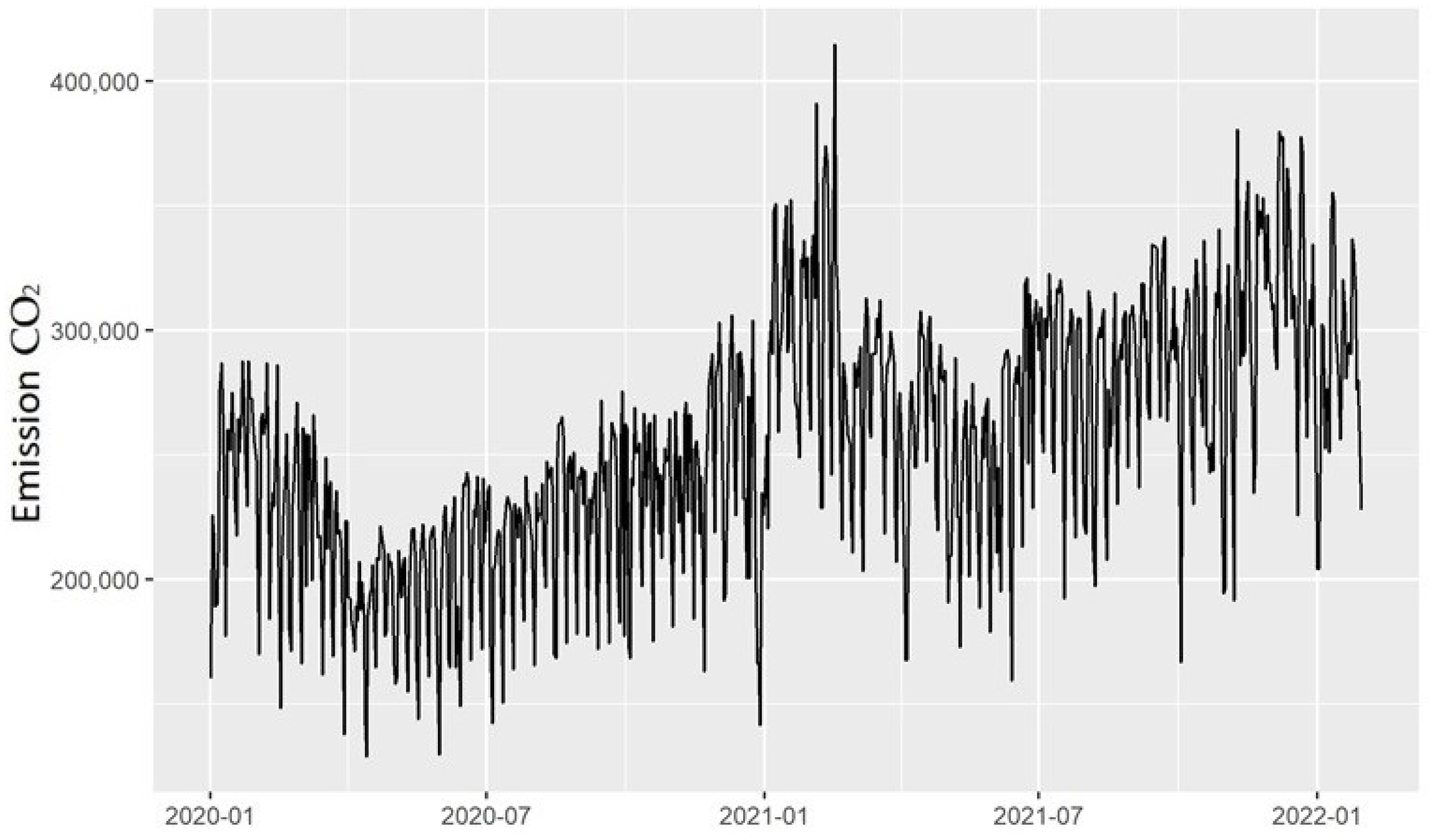
The study sample consisted of observations of CO2 emissions (Figure 1). The data were taken from the National Centre for Balancing and Emission Management (KOBiZE) for the period from 1 January 2020 to 30 January 2022. On their basis, a time series of CO2 emissions was identified, proposing a model that takes into account the seasonality of the phenomenon in relation to the month of emission and the intensity of the pandemic defined by the COVID-19 wave.
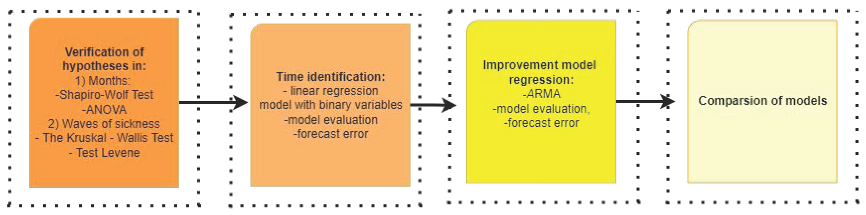
The research was carried out based on the algorithm presented in Figure 2.
Observation time was characterized by two groups: the month of the study and the pandemic wave. The latter take into account the rapid increase in the incidence of the disease and the introduction of lockdown restrictions, which allows to distinguish the 1st, 2nd and 3rd wave and the period of “no clear wave”—this is the transition time between successive waves of the disease.
Details of the individual periods are presented in Table 1.
The study examined the amount of CO2 emissions in each time frame. In addition, limitations related to the impact of other factors, such as meteorological conditions or changes in the functioning of society due to isolation or quarantine, were assumed, since they were somewhat taken into account in the individual waves defined in Table 1. For example, deterioration of weather conditions (including the autumn–winter period) resulted in an increase in the number of cases and defined the existence of a particular pandemic wave. So did isolation and quarantine, which were imposed in particular at times of increased numbers of cases. The inclusion of such variables in the study could result in an interdependence of variables.
3.1. Monthly Seasonality Study
Following the algorithm presented in Section 2, the hypothesis of normal distribution in each group was first verified using the Shapiro–Wilk normality test. The p-value was determined for each study group independently. The results are presented in Table 2.
At a significance level of 0.01, for most groups there is no reason to reject the hypothesis of a normal distribution. Only in the groups for the months of April and July a goodness of fit was not confirmed. This was followed by a test for homogeneity of variance across groups using Levene’s test. The test statistic was F = 1.7605, p-value = 0.057; therefore, there is no basis to reject the null hypothesis. The variance across groups is homogeneous.
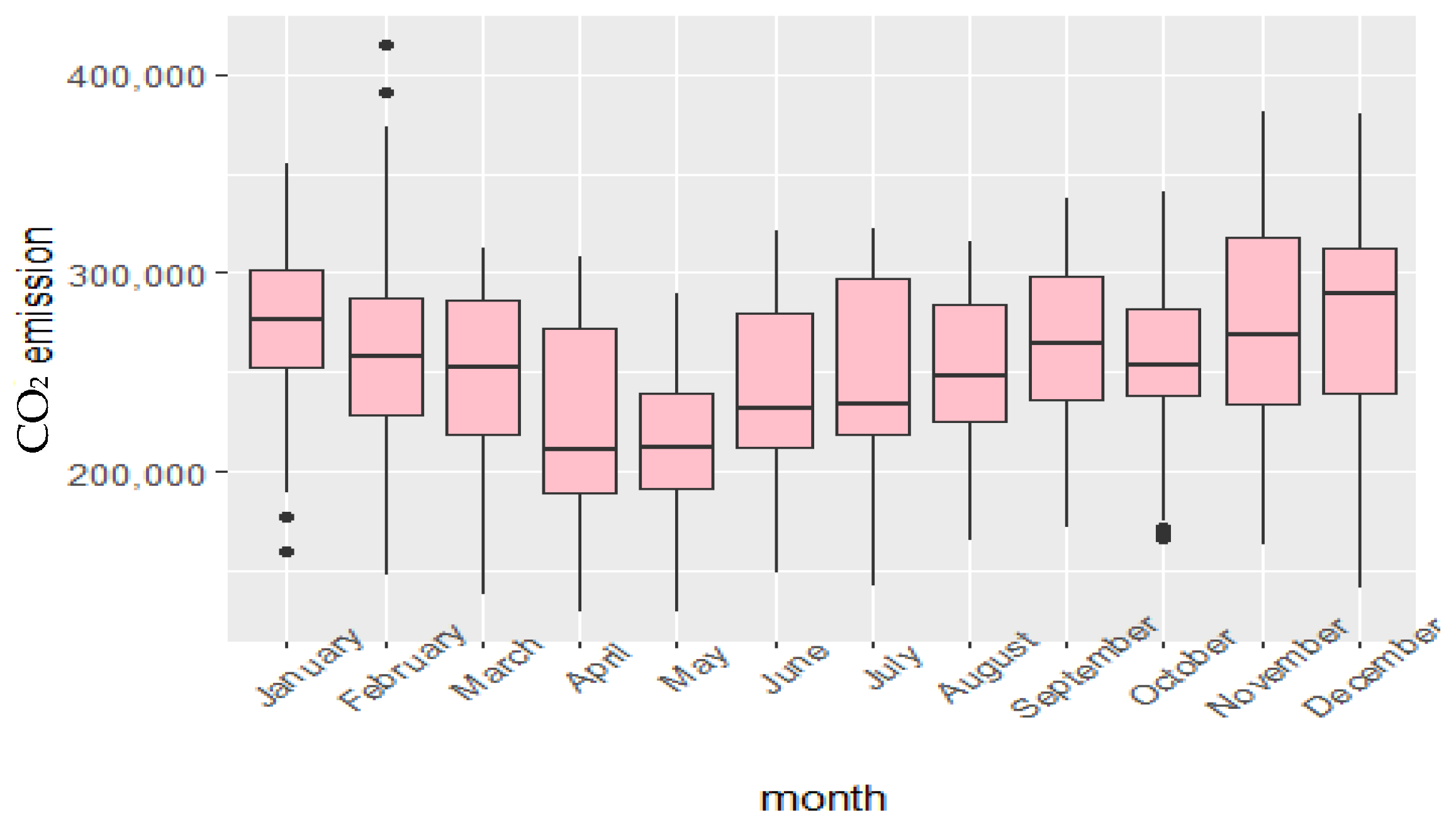
The goodness of fit of most of the empirical distributions in the groups and some robustness of the ANOVA analysis of variance to this requirement as well as confirmation of the homogeneity of the variances led to the decision to test the seasonality of monthly CO2 emissions using ANOVA. The F-test statistic was 12.54 and p-value <.
Therefore, there was no basis to accept the null hypothesis, and the difference in CO2 emissions between the months can be considered significant. This conclusion is confirmed by the box plot of the following values showing the CO2 emissions in each of the months analyzed (Figure 3)
Considering the presented results of the analysis, it can be concluded that the CO2 emissions are characterized by monthly seasonality.
3.2. Examination of the Impact of Individual COVID-19 Intensity Periods
An analogous test was performed relative to the severity of the pandemic as defined by individual waves and strolling periods (described as “no clear wave” in the table). The goodness of fit of the empirical distributions was analyzed first. At a significance level of 0.05, this assumption was confirmed for one distribution only. The results of the Shapiro–Wilk test are presented in Table 3.
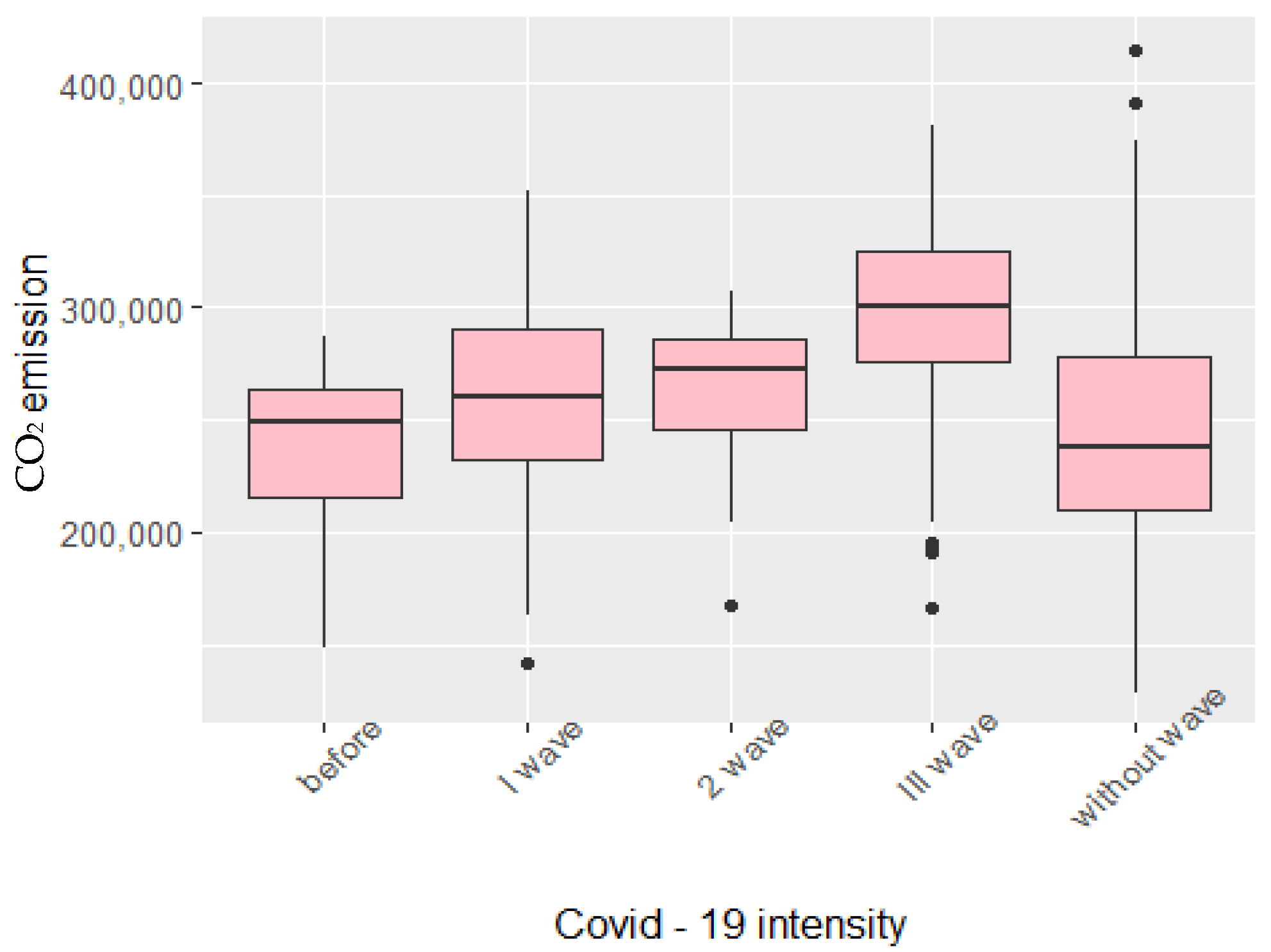
Homogeneity (equality) of variances was then checked using Levene’s test. The test statistics for the sample was F = 3.245 and the p-value = 0.012. The results obtained show a lack of homogeneity of variance across groups at a significance level of 0.05, which means that it is advisable to use the Kruskal–Wallis test. The value of calculated test statistic = 128.71, p-value < . The null hypothesis to be accepted is that the groups are significantly different. Confirmation of the test performed is shown in Figure 4. Thus, all the study variables will be used in the regression model.
4. Identification of the Time Series
4.1. Linear Regression Model
Time series identification was performed using a linear regression model with binary variables. This study uses explanatory variables that are not quantitative but qualitative in nature. Then, the set of discrete values they can take is finite; intermediate values make no substantive sense and cannot be treated in the way assumed for continuous variables. Therefore, it is necessary to re-code them into binary variables. Such a variable takes the value of 1 when the phenomenon occurs and 0 when it does not. In this case, the application of the least squares method is only possible if one of the variables from a given group is omitted from the estimation. Most often the variable with the lowest or highest mean value is selected, and then all of the other parameters are either positive or negative and refer to the level of the omitted variable. In this analysis, for the month variable, the baseline is May with the highest mean emission value and for the pre-pandemic wave variable, when the mean value was lowest. The coefficient values of the linear regression model with binary variables, estimated using the least squares method, are shown in Table 4.
Model Evaluation
The model was evaluated by checking the normality of the distribution of residuals, its stationarity and autocorrelation. Goodness of fit was checked using the Shapiro-Wilk test. The test result W = 0.027, and the p-value = 0.186 at the significance level α = 0.05 are the basis for concluding that the distribution follows a normal distribution.
The stationarity of the distribution of residuals was then tested. The KPSS and ADF test were used for this purpose. In the KPPS test, the null hypothesis is that the series under study is stationary while in the ADF test H0 assumes that the residuals do not exhibit stationarity. The value of the statistic for KPSS = 0.06 and p-value = 0.1, which means that there are no grounds to reject the null hypothesis of stationarity of the series of residuals. For the ADF test, the null hypothesis is that the distribution is stationary. The value of test statistic ADF = −6.6912 and p = 0.01, which means that there are no grounds to reject the null hypothesis.
Autocorrelation of residuals was tested using the Box-Ljung test for which the null hypothesis is that the autocorrelations for all lags are zero. The test statistic was = 250.5 and p-value < , which means that there are significant autocorrelations in the series of residuals.
4.2. ARMAX Model
Improvement of the regression model was proposed by identifying the residuals using ARMA series. Using Akaike’s criterion, individual model parameters were selected in such a way so as to produce the lowest value. External regressors associated with Covid wave and month were also included. This yielded the ARMAX (5,0,3) model whose parameters are presented below (Table 5).
As a further test, the autocorrelation of the residuals of the proposed model was again evaluated by testing the goodness of fit, stationarity and autocorrelation.
The goodness of fit was tested using the Shapiro–Wilk test. The test result W = 0.997, p-value = 0.192, does not warrant rejection of the null hypothesis. The distribution follows a normal distribution.
Stationarity of the distribution of the residuals was checked using the KPSS test and the ADF test. The value of the test statistic is for KPSS = 0.101, p = 0.1, and for the ADF test = −7.607 and p = 0.001. The test values obtained allow us to conclude that the residues exhibit stationarity.
The Box–Lijung test this time confirmed the absence of autocorrelation in the distribution of residuals value of the test statistic = 1.339, p-value = 0.247. The model can be considered correct.
Finally, a comparison of the proposed models was made using forecast errors and the Akaike criterion. The results are presented in Table 6.
5. Discussion of results and Conclusions
Global CO2 emissions from energy in 2021 were the highest on record, reaching 36.3 billion metric tons, which means a 6% increase [36]. There is no doubt that the COVID-19 pandemic contributed to this, as also confirmed by this study. It is therefore necessary and indisputable to take corrective and preventive action to ensure that the global increase in emissions in 2021 was a one-off and would not happen again. Therefore, environmental issues are an integral part of the public debate, and in the face of the COVID-19 pandemic, questions about the future of the environment started to be asked more often and more clearly, forcing governments to develop specific ideas and solutions, including those favoring the reduction of CO2 emissions.
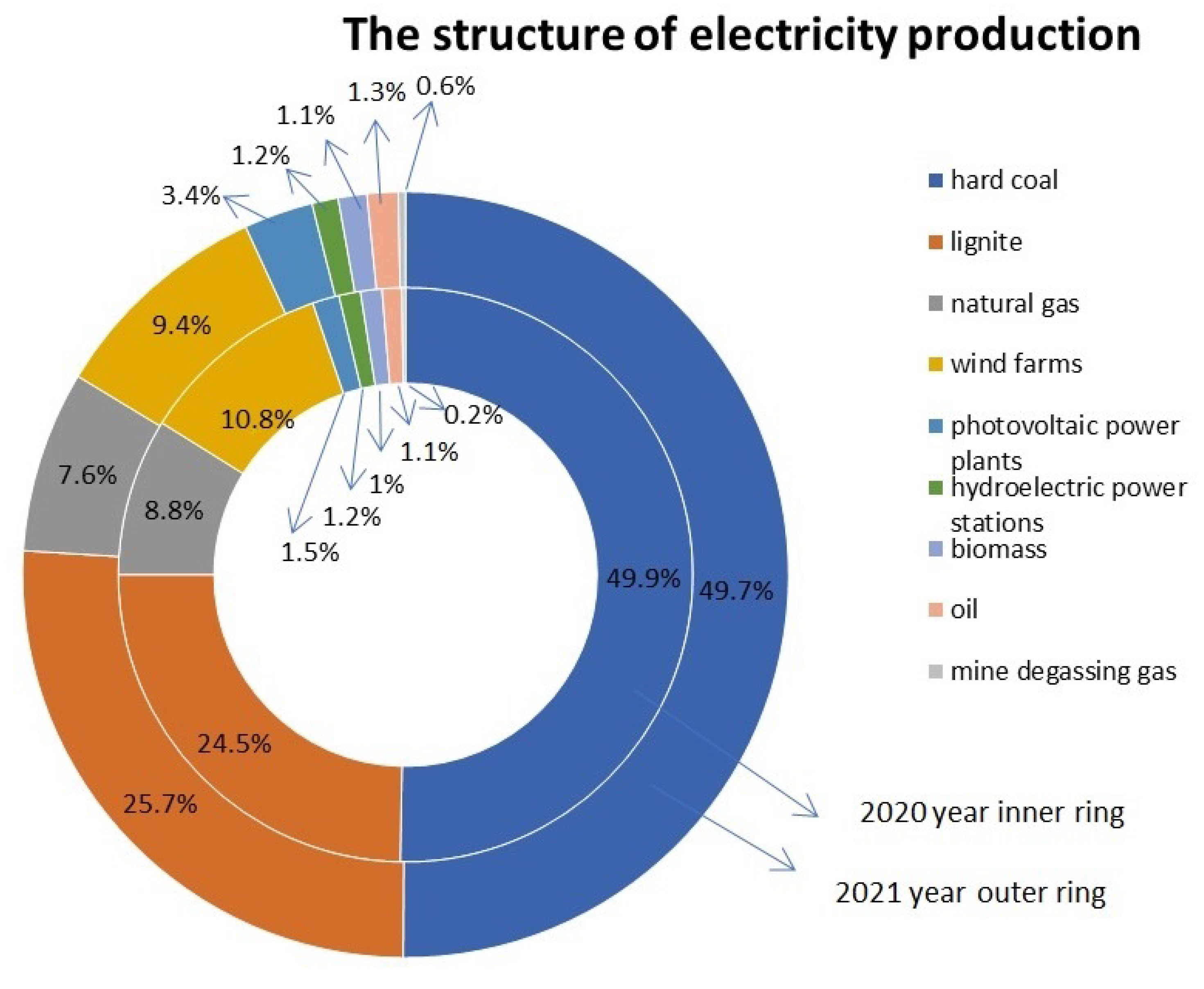
Charges resulting from CO2 emissions, which are the most important tool for achieving a 55% net emissions reduction target by 2030 in the EU, of which Poland is also a member, are to be of key importance in achieving the assumed decarbonization goals. However, penalties alone will not be effective unless governments implement comprehensive solutions to reduce CO2 emissions. The main measures should focus on increasing energy generation from green, renewable energy sources (RES) and minimizing the use of fossil fuels, as the energy sector is the main source of such high emissions. They should be adapted to the possibilities of a given country and take into account its geographical location and the possibilities of using selected energy sources. In Poland, which is discussed in this paper, renewable energy sources account for 30.3% of the installed capacity (of 55.96 GW) (data for 2021 [37]). Alternative energy sources in Poland include mainly wind energy (7.1 GW) and photovoltaics (7.7 GW). The current structure of the use of individual energy sources is presented in Figure 6.
Although the carbon footprint of electricity production in Poland is decreasing and the share of green energy is increasing, these changes are not satisfactory. It is estimated (on the basis of data published by ENTSO-E [38]) that with the recent pace of transformation towards “net zero” emissions in Poland, the climate neutrality target will be reached in 2130. The economic and environmental impacts caused by this state of affairs are worrying, especially when viewed from the perspective of the last three years disrupted by the pandemic, as this study also emphasizes.
This is why the right political decisions at the national, European and global level are crucial, not only as an opportunity to reduce emissions, but also as a development impulse for the Polish economy. These include:
- -
- systematically connecting new RES sources and other generation sources to the grid (increasing investments in this area and including them in long-term plans);
- -
- leveraging the change of priorities in the European energy sector as a development opportunity for the Polish economy;
- -
- preparing the energy system for the operation of variable sources, so that it can operate safely in any situation (e.g., lack of power from a given source);
- -
- ensuring high flexibility of the energy system in order to react actively and efficiently to changes on the supply and demand side;
- -
- creating and developing possibilities of investment financing by entrepreneurs, legal support regulations, administrative and procedural facilitation.
The above leads to the conclusion that research in the field of energy and related CO2 emission is an important element in shaping policies and attitudes consistent with sustainable development of individual states. Therefore, the assessment of factors that may affect increased emissions is very important. It was also carried out in this paper.
The hypothesis of the presented analysis was that the COVID-19 variable affects carbon dioxide emissions from electricity generation. Selected time series forecasting methods were used in the model. Initially, it was a linear regression model with binary variables and then after evaluating the residuals of the model, i.e., their normal distribution, stationarity and presence of autocorrelation, it was decided that the ARMAX model would be used.
The analysis showed that in successive months and periods of the COVID-19 pandemic, the CO2 emissions varied, and the scale of changes was clearly related to the increase in infections and disease cases, identified by the authors as successive waves of the pandemic. It turned out that an increase in incidence resulted in higher CO2 emissions each time.
Referring to the results obtained in the literature, it can be considered that they overlap in some areas with the analyses carried out by other authors, which indicate an increase in CO2 emissions from traditional sources during the pandemic due to delays in renewable energy supply chains [39], a decrease in RES investments and a shift in funding towards pandemic-related aid activities [40].
It should be stressed, however, that, contrary to the analyzed literature [41,42,43,44], an increase in CO2 emissions was recorded in the case of Poland, which somewhat differs from global trends that signaled a decrease resulting from the global energy, financial and health crises, including, inter alia, sudden stoppage of production [41], blockades related to COVID-19 [42], economic downturn [43,44], etc. The same conclusions are also provided by the reports, which indicate that while there was a global decrease in CO2 emissions in the world, an increase of 17% was recorded in the European Union in the analyzed period, mainly due to coal-fired power plants operating in Poland and Germany [45]. It should be emphasized that the analyzed Bełchatów power plant is the largest unit generating electricity from lignite in Poland and one of the largest in the world. The above confirms the validity of the results obtained by the authors.
It is worth mentioning that the highest increase in CO2 emissions was recorded for the second wave of infections. Unquestionably, this was caused by the economic recovery after the first phase of the COVID-19 pandemic. It is also worth noting that a specific situation occurred in Poland during the pandemic. The vast majority of citizens, as a result of quarantine, isolation or infection (amplified in the “autumn–winter” season) or remote work, stayed at home (generating energy needs), while workplaces functioned almost unchanged, with virtually the same demand for electricity. Examples include universities, where teachers were conducting classes in the form of e-learning, or factories, where mainly administration department employees worked from home. In addition, by far the higher consumption was recorded in hospitals, which recorded multiple increases in activity [46]. It can therefore be concluded that there was an increase in energy consumption due to the division of labor and the increased number of isolated or sick people. Moreover, the increase in CO2 emissions from fossil fuels was also influenced by rising gas prices. More expensive fuel was replaced by cheaper ones [47].
The study therefore shows that the decrease in CO2 emissions due to crisis situations, such as the pandemic analyzed here, may only be apparent. The need to diversify power sources, the decrease in investment in renewable energy sources, remote working and increased healthcare activities may all contribute to an increase in emissions of this harmful compound, as this article shows. As part of further research, individual major energy consumers can be considered in detail in order not only to identify the main source of the problem, but also to prepare targeted solutions to reduce CO2 emissions.
Author Contributions
Conceptualization, A.B., A.J. and R.P.; methodology, A.B.; software, R.P.; validation, A.J., A.B. and R.P.; formal analysis, A.B.; investigation, A.J.; resources, A.B.; data curation, R.P.; writing—original draft preparation, A.B., A.J. and R.P.; writing—review and editing, A.B., A.J. and R.P.; visualization, A.J.; supervision, A.B.; project administration, R.P. All authors have read and agreed to the published version of the manuscript.
Funding
This research received no external funding.
Institutional Review Board Statement
Not applicable.
Informed Consent Statement
Not applicable.
Data Availability Statement
Not applicable.
Conflicts of Interest
The authors declare no conflict of interest.
References
- Mongo, M.; Belaïd, F.; Ramdani, B. The effects of environmental innovations on CO2 emissions: Empirical evidence from Europe. Environ. Sci. Policy 2021, 118, 1–9. [Google Scholar] [CrossRef]
- Thonemann, N. Environmental impacts of CO2-based chemical production: A systematic literature review and meta-analysis. Appl. Energy 2020, 263, 114599. [Google Scholar] [CrossRef]
- Qingquan, J.; Khattak, S.I.; Ahmad, M.; Ping, L. A new approach to environmental sustainability: Assessing the impact of monetary policy on CO2 emissions in Asian economies. Sustain. Dev. 2020, 28, 1331–1346. [Google Scholar] [CrossRef]
- Bukowski, M.; Majewski, J.; Sobolewska, A. Macroeconomic Electric Energy Production Efficiency of Photovoltaic Panels in Single-Family Homes in Poland. Energies 2020, 14, 126. [Google Scholar] [CrossRef]
- Kędzierski, M.; Możdżeń, M.; Oramus, M. Analiza wpływu restrykcji na epidemię, mobilność i zużycie energii. In Proceedings of the Epidemia koszty i korzyści, Kraków, Poland, 12 October 2020. [Google Scholar]
- Maital, S.; Barzani, E. The global economic impact of COVID-19: A summary of research. Samuel Neaman Inst. Natl. Policy Res. 2020, 2020, 1–12. [Google Scholar]
- Aday, S.; Aday, M.S. Impact of COVID-19 on the food supply chain. Food Qual. Saf. 2020, 4, 167–180. [Google Scholar] [CrossRef]
- Rahman, M.K.; Gazi, M.A.I.; Bhuiyan, M.A.; Rahaman, M.A. Effect of Covid-19 pandemic on tourist travel risk and management perceptions. PLoS ONE 2021, 16, e0256486. [Google Scholar] [CrossRef]
- Wang, Y. Government policies, national culture and social distancing during the first wave of the COVID-19 pandemic: International evidence. Saf. Sci. 2021, 135, 105138. [Google Scholar] [CrossRef]
- Grix, J.; Brannagan, P.M.; Grimes, H.; Neville, R. The impact of Covid-19 on sport. Int. J. Sport Policy Politics 2021, 13, 1–12. [Google Scholar] [CrossRef]
- Smith, J.A.; Hopkins, S.; Turner, C.; Dack, K.; Trelfa, A.; Peh, J.; Monks, P.S. Public health impact of mass sporting and cultural events in a rising COVID-19 prevalence in England. Epidemiol. Infect. 2022, 150, 1–19. [Google Scholar] [CrossRef]
- Sahu, P. Closure of universities due to coronavirus disease 2019 (COVID-19): Impact on education and mental health of students and academic staff. Cureus 2020, 12, e7541. [Google Scholar] [CrossRef] [PubMed] [Green Version]
- Tadesse, S.; Muluye, W. The impact of COVID-19 pandemic on education system in developing countries: A review. Open J. Soc. Sci. 2020, 8, 159–170. [Google Scholar] [CrossRef]
- Karabag, S.F. An unprecedented global crisis! The global, regional, national, political, economic and commercial impact of the coronavirus pandemic. J. Appl. Econ. Bus. Res. 2020, 10, 1–6. [Google Scholar]
- van Holm, E.J.; Monaghan, J.; Shahar, D.C.; Messina, J.P.; Surprenant, C. The impact of political ideology on concern and behavior during COVID-19. J. SSRN Electron. 2020. Available online: https://papers.ssrn.com/sol3/papers.cfm?abstract_id=3573224 (accessed on 14 June 2022).
- Gabryś, H.L. Elektroenergetyka w Polsce 2020 r. Available online: https://www.cire.pl/pliki/2/2021/en_2_2021_calosc_1_31_38.pdf (accessed on 28 May 2022).
- Vinicius, B.F.; Lígia, C.; Jorge, V.B.; Benedito, D. Future Assessment of the Impact of the COVID-19 Pandemic on the Electricity Market Based on a Stochastic Socioeconomic Model. Appl. Energy 2022, 313, 118848. [Google Scholar] [CrossRef]
- Ahmad, M.A.; Ammar, M.B.; Nawaf, F.A. Impact of COVID-19 interventions on electricity power production: An empirical investigation in Kuwait. Electr. Power Syst. Res. 2022, 205, 107718. [Google Scholar]
- Yukseltan, E.; Kok, A.; Yucekaya, A.; Bilge, E.; Agca Aktunc, M.; Hekimoglu, M. The impact of the COVID-19 pandemic and behavioral restrictions on electricity consumption and the daily demand curve in Turkey. Util. Policy 2022, 76, 101359. [Google Scholar] [CrossRef]
- Halbrügge, S.; Schott, P.; Weibelzahl, M.; Buhl, H.U.; Fridgen, G.; Schöpf, M. How did the German and other European electricity systems react to the COVID-19 pandemic? Appl. Energy 2021, 285, 116370. [Google Scholar] [CrossRef]
- Khalil, E.; Vodopivec, M.; Mejjad, N.; Joaquim, C.G.; Simonovič, S.; Boulaassal, H. COVID-19 Pandemic Consequences on Coastal Water Quality Using WST Sentinel-3 Data: Case of Tangier, Morocco. Water 2020, 12, 2638. [Google Scholar] [CrossRef]
- Bermana, J.D.; Ebisu, K. Changes in U.S. air pollution during the COVID-19 pandemic. Sci. Total Environ. 2020, 739, 139864. [Google Scholar] [CrossRef]
- Loh, H.C.; Looi, I.; Hock Ch’ng, A.S.; Goh, K.W.; Ming, L.C.; Ang, K.H. Positive global environmental impacts of the COVID-19 pandemic lockdown: A review. GeoJournal 2021, 6, 10475. [Google Scholar] [CrossRef]
- Chojnacki, B.; Harenda, K.; Poczta, P. Opinia na Temat Emisji Gazów Cieplarnianych Polski na tle Budżetu Węglowego Świata; ClientEarth: Warszawa, Poland, 2020. [Google Scholar]
- González-Estrada, E.; Cosmes, W. Shapiro–Wilk test for skew normal distributions based on data transformations. J. Stat. Comput. Simul. 2019, 89, 3258–3272. [Google Scholar] [CrossRef]
- Borucka, A. Assessment of the Influence of Selected Factors on the Wear of Braking System Components as an Element of Reliability of Means of Transport. In Proceedings of the 2019 4th International Conference on Intelligent Transportation Engineering (ICITE), Singapore, 5–7 September 2019; pp. 207–211. [Google Scholar]
- Derrick, B.; Ruck, A.; Toher, D.; White, P. Tests for equality of variances between two samples which contain both paired observations and independent observations. J. Appl. Quant. Methods 2018, 13, 36–47. [Google Scholar]
- Borucka, A. Forecasting of fire risk with regard to readiness of rescue and fire-fighting vehicles. Interdiscip. Manag. Res. XIV 2018, 14, 393–395. [Google Scholar]
- Bertinetto, C.; Engel, J.; Jansen, J. ANOVA simultaneous component analysis: A tutorial review. Anal. Chim. Acta 2020, 6, 100061. [Google Scholar] [CrossRef] [PubMed]
- Knapp, H. ANOVA and Kruskal-Wallis Test. Intermed. Stat. Using SPSS 2018, 20, 107–140. [Google Scholar]
- Rath, S.; Tripathy, A.; Tripathy, A.R. Prediction of new active cases of coronavirus disease (COVID-19) pandemic using multiple linear regression model. Diabetes & Metabolic Syndrome. Clin. Res. Rev. 2020, 14, 1467–1474. [Google Scholar]
- Montgomery, D.C.; Peck, E.A.; Vining, G.G. Introduction to Linear Regression Analysis; John Wiley Sons: New York, NY, USA, 2020. [Google Scholar]
- Nunes, M. An Introduction to Time Series Models; University of Bath: Bath, UK, 2019. [Google Scholar]
- Borucka, A.; Kozłowski, E.; Oleszczuk, P.; Świderski, A. Predictive analysis of the impact of the time of day on road accidents in Poland. Open Eng. 2021, 11, 142–150. [Google Scholar] [CrossRef]
- Global COVID-19 Registry. Available online: https://www.worldometers.info/coronavirus (accessed on 14 June 2022).
- International Energy Agency, Global Energy Review: CO2 Emission in 2021 Global Emission Rebound Sharply to Highest ever Level. Available online: https://www.iea.org/reports/global-energy-review-co2-emissions-in-2021-2 (accessed on 14 June 2022).
- Agencja Rynku Energii. Available online: https://www.are.waw.pl/badania-statystyczne (accessed on 14 June 2022).
- European Network of Transmission System Operators. Available online: https://www.entsoe.eu/about/ (accessed on 14 June 2022).
- Karmaker, C.L.; Ahmed, T.; Ahmed, S.; Ali, S.M.; Moktadir, M.A.; Kabir, G. Improving supply chain sustainability in the context of COVID-19 pandemic in an emerging economy: Exploring drivers using an integrated model. Sustain. Prod. Consum. 2021, 26, 411–427. [Google Scholar] [CrossRef]
- Birol, F. Put clean energy at the heart of stimulus plans to counter the coronavirus crisis. Int. Energy Agency 2020, 14, 1–13. [Google Scholar]
- Ivanov, D.; Dolgui, A. OR-methods for coping with the ripple effect in supply chains during COVID-19 pandemic: Managerial insights and research implications. Int. J. Prod. Econ. 2021, 232, 107921. [Google Scholar] [CrossRef]
- Liu, Z.; Deng, Z.; Davis, S.J.; Giron, C.; Ciais, P. Monitoring global carbon emissions in 2021. Nat. Rev. Earth Environ. 2022, 3, 217–219. [Google Scholar] [CrossRef] [PubMed]
- Bertram, C.; Luderer, G.; Creutzig, F.; Bauer, N.; Ueckerdt, F.; Malik, A.; Edenhofer, O. COVID-19-induced low power demand and market forces starkly reduce CO2 emissions. Nat. Clim. Change 2020, 11, 193–196. [Google Scholar] [CrossRef]
- Aktar, M.A.; Alam, M.M.; Al-Amin, A.Q. Global economic crisis, energy use, CO2 emissions, and policy roadmap amid COVID-19. Sustain. Prod. Consum. 2020, 26, 770–781. [Google Scholar] [CrossRef] [PubMed]
- EMBER. Available online: https://ember-climate.org/ (accessed on 14 June 2022).
- Güler, H.; Haykır, Ö.; Selçuk, Ö. Does the electricity consumption and economic growth nexus alter during COVID-19 pandemic? Evidence from European countries. Electr. J. 2022, 35, 107144. [Google Scholar] [CrossRef]
- Wang, Q.; Yang, X.; Rongrong, L. The impact of the COVID-19 pandemic on the energy market—A comparative relationship between oil and coal. Energy Strategy Rev. 2022, 39, 100761. [Google Scholar] [CrossRef]
Figure 1.
Emission volumes per day.

Figure 2.
Research algorithm.

Figure 3.
Box plot of CO2 emissions by month.

Figure 4.
Box plot of CO2 emissions in each pandemic wave.

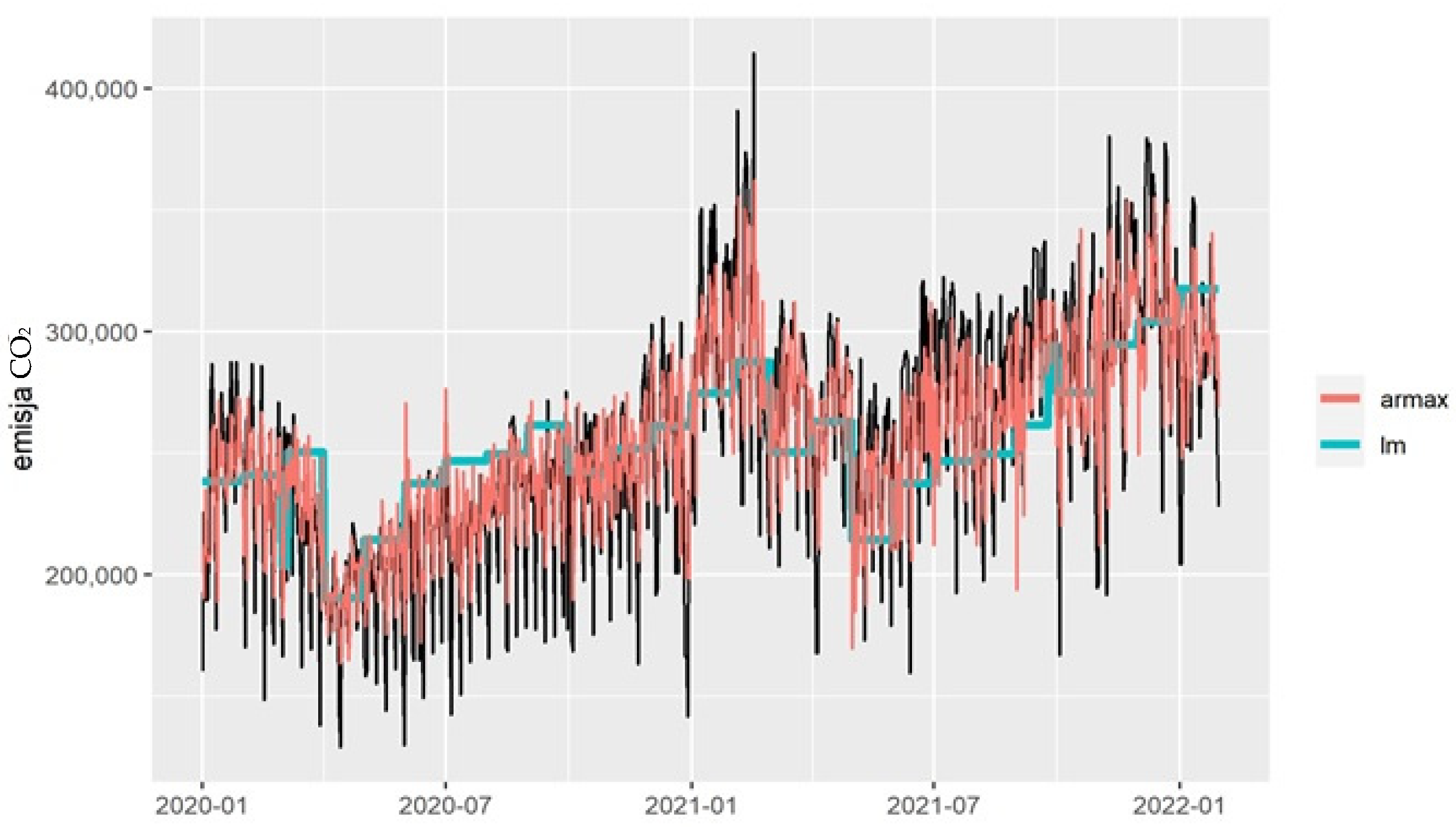
Figure 5.
Identification of CO2 emissions using a linear regression model and ARMAX model.

Figure 6.
Structure of electricity production in Poland in 2020 and 2021.


Table 1.
Characteristics of individual periods of the COVID-19 pandemic [35].
Table 1.
Characteristics of individual periods of the COVID-19 pandemic [35].
| Period Name | Date | Average Number of Cases | Average Number of Deaths | Maximum Number of Cases | Maximum Number of Deaths |
|---|---|---|---|---|---|
| 1st wave | 5 March 2020–6 June 2020 | 267 | 12 | 595 | 40 |
| 2nd wave | 24 October 2020–21 May 2021 | 15,433 | 410 | 35,251 | 954 |
| 3rd wave | 10 November 2022–24 April 2022 | 16,331 | 277 | 57,659 | 794 |
Table 2.
Shapiro–Wilk test results.
| Statistic Value | Probability | |
|---|---|---|
| January | 0.982 | 0.225 |
| February | 0.972 | 0.208 |
| March | 0.959 | 0.036 |
| April | 0.944 | 0.008 |
| May | 0.979 | 0.368 |
| June | 0.967 | 0.103 |
| July | 0.938 | 0.004 |
| August | 0.964 | 0.064 |
| September | 0.963 | 0.066 |
| October | 0.972 | 0.174 |
| November | 0.981 | 0.465 |
| December | 0.971 | 0.151 |
Table 3.
The results of the goodness of fit of the empirical distribution.
| Pandemic Stage | Statistic Value K-W | p-Value |
|---|---|---|
| Before the pandemic | 0.929 | 0.001 |
| 1st wave | 0.991 | 0.704 |
| 2nd wave | 0.887 | 0.004 |
| 3rd wave | 0.979 | 0.050 |
| no clear wave | 0.991 | 0.006 |
Table 4.
Estimated values of the parameters of the regression model.
| Variable | Estimated Value | Error | Test Statistic | p-Value |
|---|---|---|---|---|
| Absolute term | 167,537.57 | 9611.358 | 17.431 | 0.000 |
| 1st wave | 36,407.74 | 8327.012 | 4.372 | 0.000 |
| 2nd wave | 119,369.94 | 13,472.127 | 8.861 | 0.000 |
| 3rd wave | 79,384.73 | 7968.650 | 9.962 | 0.000 |
| No clear wave | 46,782.11 | 7995.977 | 5.851 | 0.000 |
| January | 70,865.23 | 9818.130 | 7.217 | 0.000 |
| February | 73,393.75 | 8751.233 | 8.386 | 0.000 |
| March | 36,098.60 | 7559.843 | 4.775 | 0.000 |
| April | −23,823.18 | 9339.370 | −2.551 | 0.011 |
| June | 23,248.41 | 7604.814 | 3.057 | 0.002 |
| July | 32,635.81 | 7542.222 | 4.327 | 0.000 |
| August | 35,399.52 | 7542.222 | 4.694 | 0.000 |
| September | 47,279.98 | 7645.214 | 6.184 | 0.000 |
| October | 28,115.14 | 8961.172 | 3.137 | 0.002 |
| November | 47,782.53 | 10,881.496 | 4.392 | 0.000 |
| December | 57,334.53 | 10,864.900 | 5.277 | 0.000 |
Table 5.
ARMAX model coefficients.
| Coefficient | Estimated Value | Coefficient | Estimated Value |
|---|---|---|---|
| Absolute term | 185,127.803 | ar1 | 1.415 |
| 1st wave | 45,728.196 | ar2 | −1.553 |
| 2nd wave | 117,671.013 | ar3 | 1.523 |
| 3rd wave | 74,828.314 | ar4 | −0.832 |
| No clear wave | 38,345.929 | ar5 | 0.321 |
| January | 43,296.255 | ma1 | −0.721 |
| February | 65,280.832 | ma2 | 0.838 |
| March | 35,385.390 | ma3 | −0.639 |
| April | −28,355.875 | ||
| May | 14,075.562 | ||
| June | 13,756.313 | ||
| July | 28,329.409 | ||
| August | 26,769.604 | ||
| September | 14,932.943 | ||
| October | 30,743.851 | ||
| November | 31,273.756 | ||
| December | 185,127.803 | ||
Table 6.
Comparison of models.
| Model Type | AIC | MAE | MPE | MAPE | MASE |
|---|---|---|---|---|---|
| Regression with binary variables | 18,355.4 | 41,548.93 | −2.981 | 14.054 | 0.816 |
| ARMAX | 17,965.9 | 25,010.6 | −1.715 | 10.477 | 0.871 |
Publisher’s Note: MDPI stays neutral with regard to jurisdictional claims in published maps and institutional affiliations. |
© 2022 by the authors. Licensee MDPI, Basel, Switzerland. This article is an open access article distributed under the terms and conditions of the Creative Commons Attribution (CC BY) license (https://creativecommons.org/licenses/by/4.0/).
Share and Cite
MDPI and ACS Style
Jaroń, A.; Borucka, A.; Parczewski, R. Analysis of the Impact of the COVID-19 Pandemic on the Value of CO2 Emissions from Electricity Generation. Energies 2022, 15, 4514. https://doi.org/10.3390/en15134514
AMA Style
Jaroń A, Borucka A, Parczewski R. Analysis of the Impact of the COVID-19 Pandemic on the Value of CO2 Emissions from Electricity Generation. Energies. 2022; 15(13):4514. https://doi.org/10.3390/en15134514
Chicago/Turabian StyleJaroń, Agata, Anna Borucka, and Rafał Parczewski. 2022. "Analysis of the Impact of the COVID-19 Pandemic on the Value of CO2 Emissions from Electricity Generation" Energies 15, no. 13: 4514. https://doi.org/10.3390/en15134514
Note that from the first issue of 2016, this journal uses article numbers instead of page numbers. See further details here.