the Creative Commons Attribution 4.0 License.
the Creative Commons Attribution 4.0 License.
 | 06 Apr 2022
Ozone pollution during the COVID-19 lockdown in the spring of 2020 over Europe, analysed from satellite observations, in situ measurements, and models
Lorenzo Costantino
Matthias Beekmann
Guillaume Siour
Laurent Menut
Bertrand Bessagnet
Tony C. Landi
Gaëlle Dufour
Maxim Eremenko
We present a comprehensive study integrating satellite observations of ozone pollution, in situ measurements, and chemistry-transport model simulations for quantifying the role of anthropogenic emission reductions during the COVID-19 lockdown in spring 2020 over Europe. Satellite observations are derived from the IASI+GOME2 (Infrared Atmospheric Sounding Interferometer + Global Ozone Monitoring Experiment 2) multispectral synergism, which provides better sensitivity to near-surface ozone pollution. These observations are mainly analysed in terms of differences between the average on 1–15 April 2020, when the strictest lockdown restrictions took place, and the same period in 2019. They show clear enhancements of near-surface ozone in central Europe and northern Italy, as well as some other hotspots, which are typically characterized by volatile organic compound (VOC)-limited chemical regimes. An overall reduction of ozone is observed elsewhere, where ozone chemistry is limited by the abundance of NOx. The spatial distribution of positive and negative ozone concentration anomalies observed from space is in relatively good quantitative agreement with surface in situ measurements over the continent (a correlation coefficient of 0.55, a root-mean-squared difference of 11 ppb, and the same standard deviation and range of variability). An average difference of ∼ 8 ppb between the two observational datasets is observed, which can partly be explained by the fact the satellite approach retrieves partial columns of ozone with a peak sensitivity above the surface (near 2 km of altitude over land and averaging kernels reaching the middle troposphere over ocean).
For assessing the impact of the reduction of anthropogenic emissions during the lockdown, we adjust the satellite and in situ surface observations for subtracting the influence of meteorological conditions in 2020 and 2019. This adjustment is derived from the chemistry-transport model simulations using the meteorological fields of each year and identical emission inventories. Using adjustments adapted for the altitude and sensitivity of each observation, both datasets show consistent estimates of the influence of lockdown emission reduction. They both show lockdown-associated ozone enhancements in hotspots over central Europe and northern Italy, with a reduced amplitude with respect to the total changes observed between the 2 years and an overall reduction elsewhere over Europe and the ocean. Satellite observations additionally provide the ozone anomalies in the regions remote from in situ sensors, an enhancement over the Mediterranean likely associated with maritime traffic emissions, and a marked large-scale reduction of ozone elsewhere over ocean (particularly over the North Sea), in consistency with previous assessments done with ozone sonde measurements in the free troposphere.
These observational assessments are compared with model-only estimations, using the CHIMERE chemistry-transport model. Whereas a general qualitative consistency of positive and negative ozone anomalies is observed with respect to observational estimates, significant changes are seen in their amplitudes. Models underestimate the range of variability of the ozone changes by at least a factor 2 with respect to the two observational datasets, both for enhancements and decreases of ozone. Moreover, a significant ozone decrease observed at a large hemispheric scale is not simulated since the modelling domain is the European continent. As simulations only consider the troposphere, the influence from stratospheric ozone is also missing. Sensitivity analyses also show an important role of vertical mixing of atmospheric constituents, which depends on the meteorological fields used in the simulation and significantly modify the amplitude of the changes of ozone pollution during the lockdown.
- Article
(3800 KB) -
Supplement
(2427 KB) - BibTeX
- EndNote


During boreal springtime of 2020, worldwide measures for curbing the spread of the COVID-19 virus have led to unprecedented and abrupt lockdowns in transportation (road, aeroplanes, and ships) and industry. These strong limitations drastically reduced the emissions of anthropogenic pollutants, inducing significant changes in atmospheric composition and air quality from local to worldwide scales, and particularly in regions such as China (e.g. Le et al., 2020) and Europe (e.g. Menut et al., 2020). Gkatzelis et al. (2021) provided an exhaustive overview of the current understanding of the influence of emission reductions due to the lockdown throughout the world on atmospheric pollutant concentrations, where air quality is described in terms of nitrogen dioxide (NO2), particulate matter (PM2.5), ozone (O3), ammonia, sulfur dioxide (SO2), black carbon, volatile organic compounds (VOCs), and carbon monoxide (CO).
Numerous efforts have been made to document and quantify the reduction in the atmospheric abundance of primary air pollutants, such as nitrogen oxides NOx (NO+NO2) and sulfur oxides SOx (SO2 + H2SO4), which are directly emitted to the atmosphere. Satellite measurements derived from the TROPOspheric Monitoring Instrument (TROPOMI) and Ozone Monitoring Instrument (OMI) have shown reductions in NO2 total columns of about 30 %–40 % over Chinese, European, and North American source regions (e.g. Bauwens et al., 2020; Muhammad et al., 2020; Le et al., 2020; Potts et al., 2021) during the pandemic lockdown. Surface in situ measurements have also revealed clear reductions in the same order of magnitude of NO2 (e.g. Ordóñez et al., 2020; Barré et al., 2021) and SO2 (e.g. Le et al., 2020).
Modelling approaches based on the construction of emission inventories accounting for the changes in anthropogenic activities have also shown consistent reduction of these primary pollutants (NOx and SOx) but also different regional regimes of either decreases or increases in the amounts of secondary pollutants, which are produced by photochemical reactions in the atmosphere (e.g. Le et al., 2020; Menut et al., 2020; Giani et al., 2020). This more complex picture is shown for secondary aerosols (organic or inorganic species) and tropospheric ozone.
An enhancement of the production of secondary particles has been linked to the alteration of atmospheric oxidizing capacity during the pandemic lockdowns (Le et al., 2020). However, the total amount of aerosols, which partly have primary origin, has shown an overall reduction in terms of PM2.5 (particle matter with aerodynamic diameter less than 2.5 µm) by roughly 5 %–10 % over Europe and 10 %–20 % over China, during the 2020 springtime lockdown period.
On the other hand, ozone pollution either decreased or increased due to the reduction in the emissions of primary pollutants, depending on the photochemical regime. This has been shown by modelling and in situ observational studies, both in China and Europe (e.g. Le et al., 2020; Shi and Brasseur, 2020; Giani et al., 2020; Souri et al., 2021; Mertens et al., 2021; Nussbaumer et al., 2021). Ozone decreased in rural areas, where photochemical production of ozone is controlled by the abundance of nitrogen oxides (thus a NOx-limited regime), the concentrations of which clearly decreased during the pandemic lockdown. Ozone pollution was clearly enhanced in urban areas (Ordóñez et al., 2020) and particularly in megacities (Sicard et al., 2020), as the reduction of NO2 amounts strongly inhibited night-time titration. The reduction of this dominant sink led to accumulation and therefore enrichment of ozone, which prevailed over the reduction of ozone production associated with the lack of precursors. Although these processes have been observed in previous works, the quantification of them is complex and it remains a challenge, as well as the precise areas over which different regimes have prevailed. An additional major factor affecting the abundance of ozone, which adds complexity to its analysis, is the meteorological conditions. Using in situ surface observations and a predictive model of ozone variation against meteorological conditions, Ordóñez et al. (2020) suggested that clear-sky conditions and relatively high surface temperature in April 2020 as compared to previous years induced intense ozone enhancements (in terms of daily 8 h maximum) over northern Europe, comparable and even larger than the enhancement associated with the pollutant emission changes linked to the pandemic lockdowns. Based on observation and meteorological analysis over the last 7 years Deroubaix et al. (2021) suggested that the total oxidant concentrations (Ox + O3 + NO2) decreased in southwestern Europe while they remained unchanged in northern Europe. Using a chemistry-transport model with emission adjusted with respect to satellite measurements of NO2 and formaldehyde, Souri et al. (2021) suggest a significant role of meteorological conditions but smaller than that associated with anthropogenic emission changes during lockdowns (58 % of the ozone enhancement, where it is 42 % for meteorology change between 2020 and 2019). Moreover, a larger-scale study based on ozone measurements from in situ sondes and lidars observed a reduction of free troposphere ozone across the Northern Hemisphere of about 7 % (4 ppb) due to worldwide activity reduction during spring and summer 2020 (Steinbrecht et al., 2021). It is worth noting that none of these studies have used satellite measurements of ozone concentrations themselves as a complementary source of information.
The present work presents the first study integrating satellite ozone observations of lowermost tropospheric (LMT) ozone, surface in situ measurements, and chemistry-transport modelling for analysing the reductions and enhancements of ozone pollution over Europe associated with the COVID-19 lockdown of spring 2020. We use satellite measurements derived from the IASI+GOME2 (Infrared Atmospheric Sounding Interferometer + Global Ozone Monitoring Experiment 2) multispectral synergism, which provides currently unmatched sensitivity to near-surface ozone (Cuesta et al., 2018). The sensitivity of this satellite retrieval shows a relative maximum for ozone around 2.2 km of altitude over land (while it is typically above 3 km for other standard satellite approaches; see details in Cuesta et al., 2013, 2018). It offers a full cloud-free spatial coverage, which is complementary to in situ measurements. We also use the chemistry-transport model CHIMERE (Menut et al., 2013; Mailler et al., 2017) for assessing the consistency of this model with respect to the observations and to analyse the influence of meteorological conditions in 2020 as compared to 2019 (the year used as baseline or standard conditions in this study). The consistency of satellite data and simulations is analysed with respect to the Air Quality e-Reporting database providing near-real-time air-quality measurements in Europe. Section 2 of the paper describes these datasets and the strategy used for their analysis. Section 3 presents the results, first in terms of total differences between 2020 and 2019, secondly the influence of meteorological conditions, and finally the impact of the COVID-19 lockdown on ozone pollution. Additional discussions on anthropogenic emissions and meteorological conditions are also given in Sect. 4. A sensitivity study shown in the Supplement of the current paper considers a different setup of the CHIMERE model, in terms of emission inventories and meteorological models, for analysing possible uncertainties in the simulations. A last Sect. 5 provides the conclusions of this work.
Being a secondary and reactive pollutant, the analysis of tropospheric ozone is complex since it is influenced by many competing factors. Tropospheric ozone sources and sinks are affected by multiple photochemical processes and non-linear effects, which vary in time and space according to the availability of different precursors, either NOx or VOC (originating themselves from multiple anthropogenic and natural sources) and meteorological conditions. An integrated approach including multiple datasets of different kinds is therefore valuable for better understanding the evolution of this pollutant. In the current study, we use both satellite and in situ surface data to quantify the difference between the ozone pollution observed over Europe in spring 2020 with respect to that in spring 2019, which is affected by both the lockdown reduction of pollutant emissions and meteorological conditions. First, we verify the consistency of these observations with respect to simulations from CHIMERE. This model simulates the 2 years, with a standard or business-as-usual inventory for 2019 and a modified version in 2020 accounting for the lockdown conditions, hereafter referred to as STD and COVID, respectively. Second, we use the chemistry-transport model with the same inventory (standard) for both years, 2020 and 2019, to derive a first-order adjustment for accounting for the influence on ozone pollution of the change in meteorological conditions between the 2 years. This allows us to obtain an approximate estimate of the effects of the COVID-19 lockdown conditions on ozone pollution from the two observational datasets (in situ and satellite). This is expressed by the following equation:
where modSTD corresponds to simulated ozone with the standard or business-as-usual inventory. This adjustment does not rely on any estimation of the variations in anthropogenic emissions during the lockdown. For simulations, the superscripts 2020 and 2019 refer to the year of meteorological conditions that have been used. For observations, these superscripts indicate the year when they are performed. The same equation stands for the adjustment of both surface measurements and satellite retrievals (which are adjusted independently) but gridded at the location or horizontal resolution of each observation. The adjustments for surface measurements and satellite retrievals are different, as they use simulated ozone concentrations, respectively, at the surface and at the lowermost troposphere (LMT, below 3 km of altitude), while these last ones are smoothed by the satellite averaging kernels. The accuracy of this first-order adjustment or correction depends on the performance of the chemistry-transport model to simulate ozone concentrations in business-as-usual conditions as a function of meteorological conditions. It implicitly accounts for changes in biogenic emissions between 2020 and 2019 which are directly linked to meteorological conditions. However, this adjustment cannot account for the changes in the chemical regimes (either NOx-limited or VOC-limited) due to the changes in the abundance of ozone precursors nor other complex chemical regimes (as modelled for parts of the Po Valley, Thunis et al., 2021).
We compare this synergetic observational and model estimate with the one derived from models only, based on the difference of ozone simulations with inventories COVID and STD and the meteorological conditions of 2020, as follows:
In the current work, we mainly focus on the period from 1 to 15 April 2020 (and use 1–15 April 2019 as standard period), which corresponds to the 15 d period of most perturbed emissions by the lockdown according to the COVID emission reduction factors from CAMS (https://atmosphere.copernicus.eu/covid-data-download, last access: 1 April 2022). This work reports for example a reduction of −73 % of gasoline road transport for the five most populated countries in Europe (Germany, France, Great Britain, Italy, and Spain, which are also the largest contributors to the total European emission decreases), whereas it is −64 % and −66 % for the 15 d before and after (and then −54 % and −38 % for the two following fortnights). We also show some of the results for the whole month of April (2020 and 2019) to directly compare our estimates with those from previous works (Ordóñez et al., 2020; Souri et al., 2021) provided as monthly averages.
The following paragraphs describe briefly the datasets used by this approach.
2.1 IASI+GOME2 multispectral satellite observation of lowermost tropospheric ozone
The IASI+GOME2 satellite approach is designed for observing lowermost tropospheric ozone through the multispectral synergism of thermal infrared (IR) atmospheric radiances observed by IASI (Infrared Atmospheric Sounding Interferometer, Clerbaux et al., 2009) and ultraviolet (UV) earth reflectances measured by GOME-2 (Global Ozone Monitoring Experiment 2, EUMETSAT, 2006), according to the detailed description provided by Cuesta et al. (2013). Both instruments are aboard the MetOp satellite series, and they both offer global coverage every day (for MetOp-A, B, and C, respectively around 09:30, 09:00, and 10:00 LT) with a relatively fine ground resolution (12 km diameter pixels spaced by 25 km for IASI at nadir and ground pixels of 80 km × 40 km for GOME-2). IASI+GOME2 jointly fits co-located IR and UV spectra for retrieving a single vertical profile of ozone for each pixel. The horizontal resolution corresponds to that of IASI, using for each pixel the UV measurements from the closest GOME-2 pixel (without averaging).
The present work uses daily IASI+GOME2 multispectral observations of ozone available for clear sky and low cloudiness (pixel cloud fractions below 30 %) and derived from the average of the retrievals using measurements from all available MetOp satellites (A, B, and C for 2020 and A and B for 2019). The version of the algorithms used here is described and validated at a global scale against ozone sondes by Cuesta et al. (2018) (with a correlation of 0.85, a mean bias of −3 %, and a precision of 16 %). The capacity to observe near-surface ozone with IASI+GOME2 has been shown by a good agreement against surface in situ measurements of ozone for two major ozone outbreaks across East Asia and at a daily scale (a correlation of 0.69, a weak mean bias of −5 %, a precision of 20 %, and similar standard deviations for both datasets). Single-band approaches as those from IASI only were not able to observe such near-surface variability.
The IASI+GOME2 satellite product includes vertical profiles of ozone, partial columns, averaging kernels (representing sensitivity of the retrieval to the true atmospheric state), error estimations, and quality flags. Since 2017, global-scale IASI+GOME2 retrievals have routinely been produced by the French data centre AERIS, and they are publicly available (see https://www.aeris-data.fr, last access: 1 April 2022, and https://iasi.aeris-data.fr, last access: 1 April 2022).
2.2 Surface in situ measurements
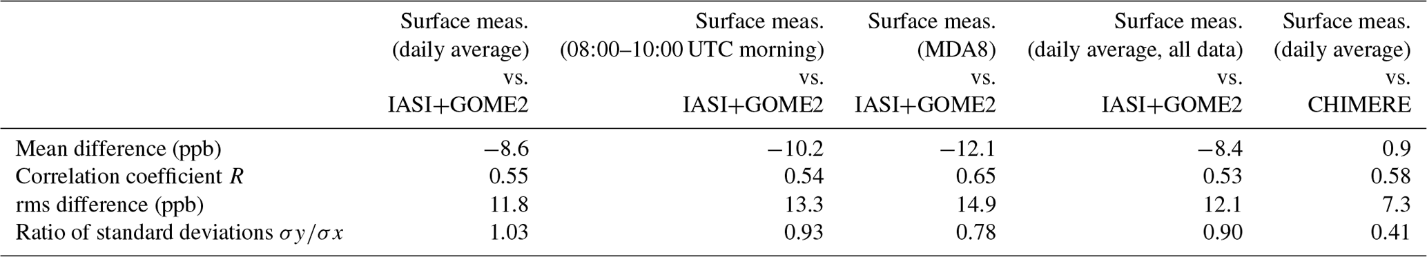
In this work, we use in situ surface measurements of O3 and NO2 from the European Air Quality e-Reporting (https://www.eea.europa.eu/data-and-maps/data/aqereporting-8, last access: 14 September 2021). We only consider background stations of all categories (urban, suburban, and rural). We mainly analyse here daily averages of surface concentrations and compare them with IASI+GOME2 ozone data and CHIMERE model simulations. For verification, we also consider morning and maximum daily averages over 8 h (MDA8) of surface concentrations. A comparison shown in Table 2 and commented in Sect. 3.1 suggests that a slight better agreement is found between daily averages of surface data (as compared to morning averages or MDA8) and IASI+GOME2. This is likely linked to the fact that IASI+GOME2 retrievals show a relative maximum of sensitivity at about 2.2 km of altitude over land in mid-latitudes (see Cuesta et al., 2013). At this altitude and during the overpass time of the MetOp satellites around 09:30 LT, the IASI+GOME2 approach likely measures ozone concentrations at the residual atmospheric boundary layer. We expect that the variability of these last ones is better represented by daily averages than morning surface concentrations, which have not yet been mixed vertically within the whole boundary layer. Surface MDA8 concentrations are closely linked with the daily maximum that occurs within the mixing boundary layer. These values show larger variability than satellite data, and their average values present greater differences than with respect to surface daily averages. Therefore, these last ones are used for comparisons with IASI+GOME2.
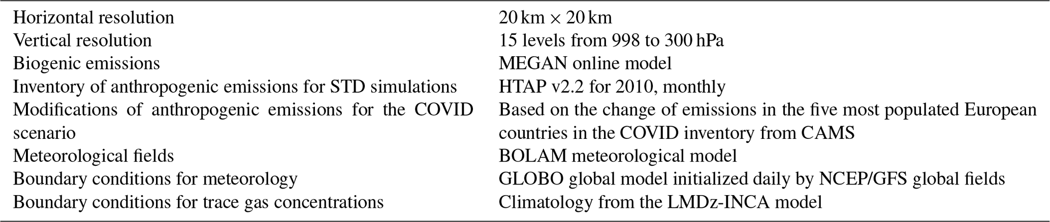
Table 1Brief description of the setup of the CHIMERE model, used for the simulations of ozone distribution over Europe in April 2019 and April 2020 (STD and COVID scenario).
2.3 CHIMERE chemistry-transport model
CHIMERE is a state-of-the-art chemistry-transport model widely used for studying atmospheric composition and forecast mainly at a regional scale (e.g. Vautard et al., 2000; Honoré et al., 2008; Rouïl et al., 2009; Menut and Bessagnet 2010; Menut et al., 2015a; Marécal et al., 2015). It has been compared to numerous measurements, including meteorological variables and atmospheric chemical species (Menut et al., 2000, 2005a, 2015b; Bessagnet et al., 2016; Vivanco et al., 2017). Regularly, new versions of the model are proposed for a community of users (Menut et al., 2013; Maillet et al., 2017). Whereas ozone and nitrogen oxides are modelled as explicit species, other species such as particulate matter or VOCs are composed by several ensembles of families of species. Biogenic emissions are estimated with the MEGAN online model (Guenther et al., 2006), mineral dust with the scheme from Alfaro and Gomes (2001) and Menut et al. (2005b), and sea salt with that from Monahan (1986).
In the present study, we use a setup of CHIMERE that offers a fair match with respect to observational datasets. These simulations are run with horizontal resolution of 20 km × 20 km and 15 vertical levels from 998 to 300 hPa. Table 1 presents a brief description of the main elements of the model.
CHIMERE uses anthropogenic emissions from the HTAP v2.2 inventory for 2010, on a monthly basis (https://edgar.jrc.ec.europa.eu/htap_v2/ last access: 14 September 2021, Janssens-Maenhout et al., 2015). The original inventory is considered for STD simulations in 2019 and 2020, whereas for the COVID emissions in 2020 a relative reduction for each activity sector (road transport, residential, industry, aviation, and shipping) is applied. The magnitude of the decrease is estimated for the European domain based on the average for the five most populated European countries (Germany, France, Great Britain, Italy, and Spain) of the CAMS COVID daily emission reduction factors for each sector, averaged over the period 1–15 April 2020. Even though some differences occur in emission variability from country to country, with Spain, Italy, and France showing the strongest changes, while Great Britain and mostly Germany show weaker ones, we assume here a spatially homogeneous variation of emission factors over the whole domain. For 1–15 April 2020, this corresponds to −73 %, −16 %, −44 %, +5 %, −91 %, and −19 % for emissions from road transport, power, industry, residential, aviation, and shipping sectors. According to CAMS, the COVID-19 restrictions led to a heterogeneous impact across different pollutants from industrial and residential sectors (https://atmosphere.copernicus.eu/emissions-changes-due-lockdown-measures-during-first-wave-covid-19-europe last access: 1 April 2022). For the industry sector, a smaller reduction is observed for non-methanic volatile organic compounds (NMVOCs), NH3, and SO2 (mostly emitted from food/beverage and chemistry industries, less affected by lockdown measures) with respect to other pollutants. For the residential sector, only those pollutants mainly related to wood combustion processes (i.e. PM10, PM2.5, NH3, NMVOC, CO, biogenic CO2, and CH4) experienced a slight increase, while NOx and SOx (as well as fossil-fuel-related CO2) showed a modest decrease. For that reason, the COVID scenario considers the partitioning for industry between NMVOCs, NH3 and SOx, as well as that for the residential sector between NOx and SOx, which are used within CAMS revised inventory.
Meteorological fields are derived with the BOLAM (e.g. Buzzi et al., 1998) hydrostatic meteorological model, whose boundary conditions are provided by the GLOBO (e.g. Malguzzi et al., 2011) hydrostatic general circulation model. Both models are developed at CNR-ISAC (https://www.isac.cnr.it/dinamica/projects/forecasts/, last access: 1 April 2022). Initial conditions of BOLAM and GLOBO are taken each day at 00:00 UTC from analyses of the NCEP/GFS model (Kalnay et al., 1996). Climatological boundary conditions of trace gas concentrations are taken from LMDz-INCA (Szopa et al., 2009; http://inca.lsce.ipsl.fr/, last access: 1 April 2022), the same for the 2 years.
In the Supplement of the present paper, we also show simulations with different anthropogenic emission inventories and meteorological conditions. They provide an estimation of the uncertainties of the ozone pollution simulations during the lockdown conditions.
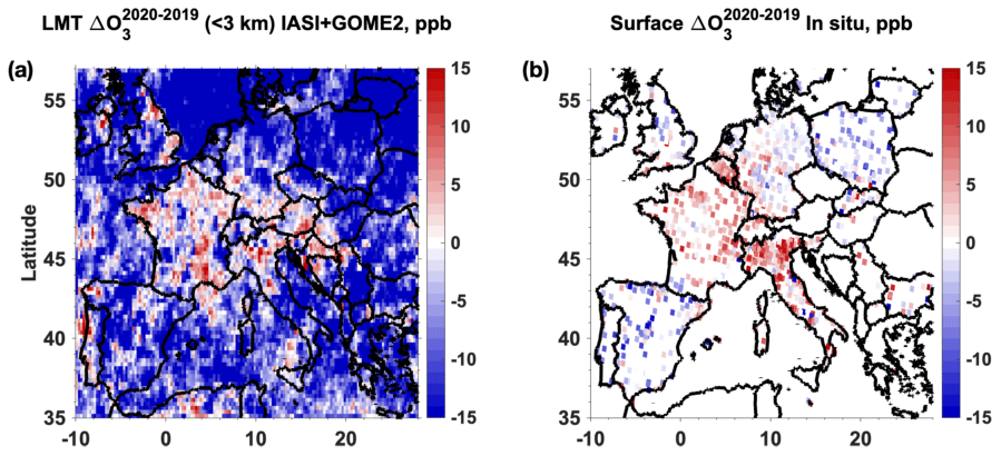
Figure 1Changes in ozone concentrations (ppb) between the average on 1–15 April 2020 and that of the same period in 2019 observed (a) at the lowermost troposphere (below 3 km of altitude) by the IASI+GOME2 multispectral satellite approach and (b) at the surface by in situ sensors from the EEA network. The temporal and spatial sampling of both datasets is the same, only considering in situ data coincident in time and space with the satellite retrievals (on a daily basis).
For better understanding the information provided by observations and simulations, the current multi-data analysis is presented in several steps. First, we focus on the total changes of ozone pollution between 2020 and 2019 (Sect. 3.1) that are directly observed by in situ sensors and from space, and which we compare with the corresponding amount simulated by the model. Then, we analyse the model-derived changes between these 2 years but only associated with meteorological conditions (Sect. 3.2). Finally, we compare changes of ozone pollution only linked with the pandemic lockdown conditions, estimated from models and observations (Sect. 3.3). The originality of these results resides in the use of in situ and satellite observational estimates of the changes in ozone pollution associated the lockdown conditions , which are adjusted for subtracting meteorology effects.
3.1 Changes in ozone pollution in 2020 with respect to 2019
3.1.1 Satellite and in situ surface measurements
The first step of our study consists of analysing all available datasets in terms of the changes in ozone pollution over Europe between the pandemic lockdown period in 2020 (focused here on 1–15 April) with respect to the same period during the previous year (this difference is hereafter called ). Figure 1 shows a comparison between the two observational datasets, while Fig. 1b only considers in situ data coincident in time and space with satellite data (although very few differences are seen for the average of the whole in situ dataset). A good agreement is shown in terms of regional ozone patterns between IASI+GOME2 satellite data and in situ surface measurements. Both datasets clearly show similar structures of positive and negative anomalies. Ozone enhancements in 2020 with respect to 2019 are seen both by satellite and surface data over northern and eastern France, western and southern Germany, northern Italy, and southwest England. Ozone photochemistry in these regions is typically dominated by VOC-limited conditions, observed both in standard situations (e.g. Beekmann and Vautard, 2010, Wilson et al., 2012) and during the pandemic lockdown (e.g. Menut et al., 2020; Gaubert et al., 2021). Both measurements also show clear ozone reductions in 2020 for less urbanized regions typically characterized by NOx-limited chemical conditions: Spain, southern Italy, Poland, and western England. A near-neutral or intermediate behaviour is seen over eastern Germany (in consistency with Beekmann and Vautard, 2010), with rather limited reductions of ozone both for IASI+GOME2 and surface data.
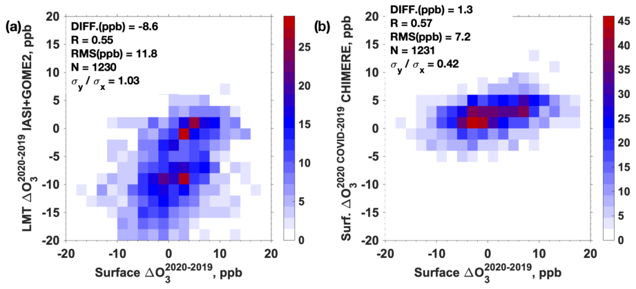
Figure 2Scatterplot of changes in ozone concentrations averaged over 1–15 April 2020 with respect to the same period in 2019 (a) at the LMT from the IASI+GOME2 satellite approach and (b) at the surface from the CHIMERE model, with respect to co-localized surface in situ measurement. The colour scale represents the number of occurrences of points within each sector of 2 ppb × 2 ppb. We consider here only in situ data coincident in time and space with the satellite retrievals.
Table 2Statistics of the comparisons of in situ surface observations with respect to IASI+GOME2 lowermost tropospheric ozone retrievals and model simulations. All surface in situ measurements and CHIMERE model simulations correspond to data coincident with IASI+GOME2 retrievals on a daily basis, except for the column “Surface meas. (daily average, all data) vs. IASI+GOME2”.
In quantitative terms, a scatterplot of co-located IASI+GOME2 and in situ data in time and space is presented in Fig. 2a. Colours represent the number of occurrences for intervals of 2 ppb of ozone in both axes. The correlation coefficient between these datasets is 0.55, while the standard deviation of both datasets is practically the same and the root-mean-squared (rms) difference is 11.8 ppb. When considering the average of the whole in situ dataset, the only notable change is an increase in the standard deviation of 13 % for the surface data (see Table 2). In all cases comparing daily averages of in situ data, there is an average difference or shift of ∼ 8.6 ppb for the average ozone concentration changes, with lower values for the satellite retrievals than those for in situ data. This difference in average concentrations may partially come from the altitudes of the measurements: in situ data are surface measurements, whereas IASI+GOME2 measurements are lowermost tropospheric ozone columns. The satellite retrieval of this partial column is typically most sensitive around 2.2 over land (quantified over Europe by Cuesta et al., 2013). Therefore, the negative difference for IASI+GOME2 with respect to surface concentrations may suggest that the reduction of ozone concentrations in 2020 with respect to 2019 at atmospheric layers roughly ∼ 2 is more important than at the surface. This could be explained by several reasons such as a larger sensitivity to emission changes at the surface than at higher altitudes, differences in sampling time, and also by the fact that satellite measurements sample air masses of both the boundary layer and free troposphere, where ozone concentrations may have had different variations between 2019 and 2020. Moreover, surface ozone concentrations are directly affected by titration with NO; its impact on ozone columns up to 3 km is expected to be lower. Since the degree of freedom for the LMT partial columns is generally lower than 1 (typically 0.35 over land in Europe), IASI+GOME2 retrievals could also have some influence of the a priori concentrations.
The observational study from Steinbrecht et al. (2021) shows a clear reduction of ozone concentrations of −6 % to −9 % in the free troposphere (1–8 km of altitude) in the extratropical Northern Hemisphere. This is mainly associated with the reduction of anthropogenic emissions at a large scale during the pandemic lockdown in 2020 and to a lower degree to a large 2020 springtime ozone depletion in the Arctic stratosphere (less than one-quarter of the observed tropospheric anomaly; see also Bouarar et al. 2021, Miyazaki et al. 2021, Ziemke et al. 2021). This large-scale reduction of ozone concentrations in the free troposphere is consistent with the negative difference of LMT ozone satellite retrievals (capturing the variability of both ozone in the boundary layer and the free troposphere; see further discussions in Sect. 4) with respect to surface ozone concentrations.
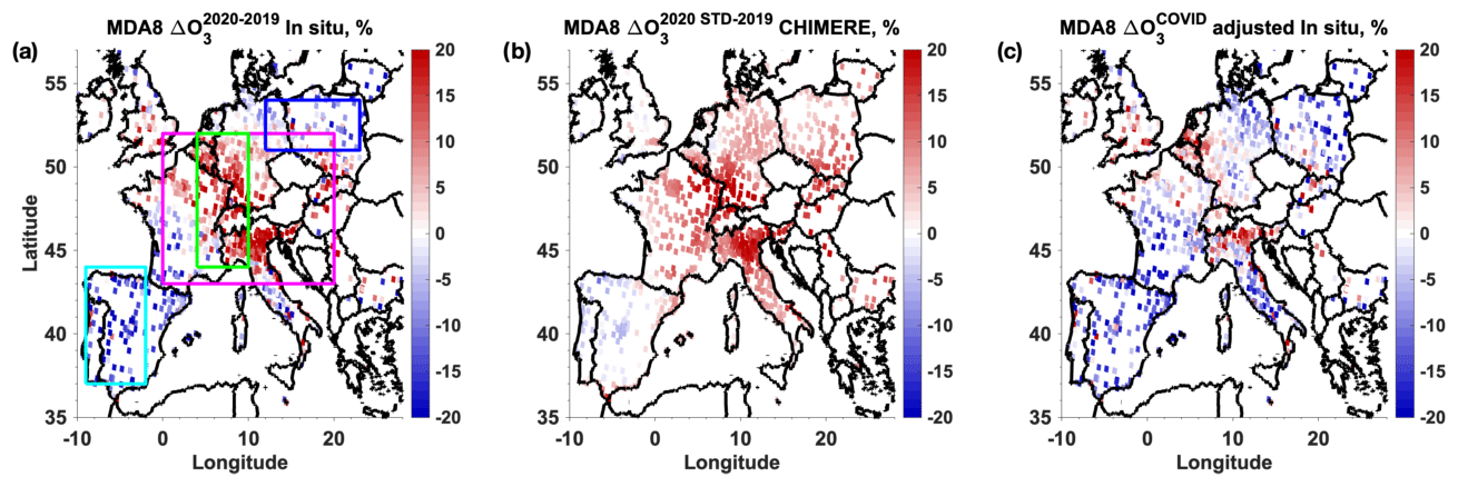
Figure 3Relative changes (in %) in maximum daily average during 8 h (MDA8) of surface ozone concentrations between 2020 and 2019, during the period 1–30 April (a) measured by in situ sensors, (b) associated with meteorological conditions derived from the difference between CHIMERE simulations in 2020 using STD emissions and 2019, and (c) related with the pandemic lockdown in 2020 measured by in situ sensors and adjusted for subtracting the effects of meteorological conditions using Eq. (1). Percentages are calculated with respect to averages for the corresponding period in 2019. Rectangles in panel (a) indicate the target regions indicated in the text and Tables 4 to 6.
Figure 3a presents the changes in ozone pollution between 2020 and 2019 but in terms of maximum 8 h average (MDA8) of surface ozone and covering the whole month of April. In Sects. 3.1 to 3.3, this amount is used for direct comparisons of the results of the present paper with two previous studies (i.e. Ordóñez et al. 2020; Souri et al., 2021). We notice that MDA8 and daily average ozone concentrations present rather similar horizontal patterns of positive and negative anomalies between the 2 years over most of Europe (central Europe, France, Spain, and Italy; see Figs. 3a and 1b), even if the averaging period slightly changes between the two figures. In quantitative terms, the MDA8 ozone concentrations changes are clearly larger than for daily averages, by about a factor ∼ 2 (see Tables S1 and S2 in the Supplement). These differences are probably linked to the fact that daily averages also account for low ozone concentrations during the night, and therefore their variability is reduced with respect to daily maxima expressed here as MDA8.
Figure 3a shows very similar horizontal patterns of positive and negative anomalies as compared with the estimate from Souri et al. (2021, Fig. 9 of this work). The average ozone change over the central Europe region (43–52∘ N, 0–20∘ E) is moderately larger in the present work (11.0 %; see Table 5) than that from Souri et al. (2021; i.e. 7.4 %), which can partly stem from the choice of surface stations considered in study. The ozone changes in April 2020 derived by Ordóñez et al. (2020, Fig. 1 of this study, e.g. +12 % to +22 % in the Benelux) are also consistent with the present work (16 % in the Benelux area; see Table 5). However, ozone enhancements extend further east (also over eastern Germany and Poland) in the estimations of Ordóñez et al. 2020 as compared to Fig. 3a. This can partly come from the fact that Ordóñez et al. 2020 use an average of 2015–2019 as standard conditions, while only 2019 is considered here.
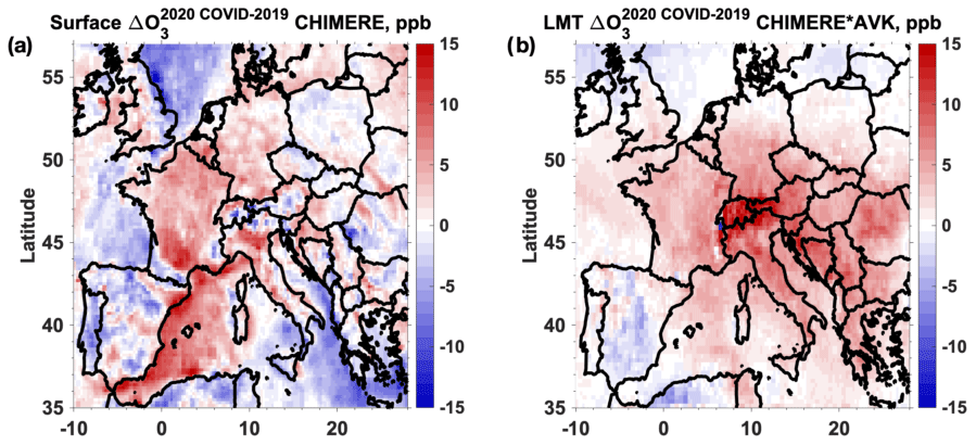
Figure 4(a) Same as Fig. 1b but for simulated surface with the CHIMERE model coincident with daily IASI+GOME2 retrievals. (b) Same as Fig. 1a but for simulated LMT (< 3 km a.s.l.) from CHIMERE smoothed by the averaging kernels of IASI+GOME2 co-located retrievals.
3.1.2 Model simulations
When it comes to model-derived changes of surface ozone concentrations between 2020 (using COVID emissions) and 2019 for 1–15 April (Fig. 4), we observe significant similarities and differences with respect to observations (Fig. 1). CHIMERE simulates ozone enhancements in 2020 with respect to 2019 over central Europe and northern Italy, as well as reductions over Spain, the Atlantic, the North Sea, and southern Italy and the central-eastern Mediterranean in consistency with most surface in situ measurements and IASI+GOME2 data. This is similarly found for LMT partial columns from CHIMERE smoothed by IASI+GOME2 averaging kernels (for accounting for the satellite vertical sensitivity, Fig. 4b), except for simulated enhancements over the Atlantic and the central-eastern Mediterranean. However, the model depicts limited changes over Poland and enhancements over eastern Europe and the western Mediterranean, whereas both observations (satellite and when available in situ) depict clear reductions in 2020 with respect to 2019. The scatterplot of Fig. 2b shows a fair correlation (0.58) of CHIMERE with respect to in situ data. However, the model clearly underestimates the variability of the ozone changes in spring 2020 with respect to the previous year, as compared to in situ measurements (larger by more than a factor ∼ 2). Whereas values observed at the surface range from roughly −12 to +12 ppb in terms of daily averages, simulated values only spread from −6 to +6 ppb. The range of values of IASI+GOME2 has the same amplitude as the in situ data but shifted towards smaller values (−20 ppb to +5 ppb).
Generally, simulations show total anomalies in 2020 (with respect to 2019) that are only partially associated with the regions of typical NOx-limited and VOC-limited chemical regimes. On the other hand, observations from both in situ sensors and satellite do show clearer similarities between the typical regimes (in the regions where both datasets are available) and ozone anomalies during the pandemic lockdown. This might be linked to a large influence of meteorological conditions in the model, as compared to lockdown-induced emission changes. Still another reason for these differences could be that boundary conditions outside the simulation domain of CHIMERE do not account for the changes in anthropogenic emissions linked with the pandemic in 2020 at a large scale. This would lead to a positive bias in simulated differences if part of the observed decrease at the free troposphere (by Steinbrecht et al., 2021) affected the surface. Overall, the differences between the model and observations highlight the complexity to simulate the effect of the changes in ozone concentrations due to changes in anthropogenic emissions, as occurred during the lockdown.
3.2 Changes in ozone pollution associated with meteorological conditions
Figure 3b shows the changes of MDA8 surface ozone in 2020 with respect to 2019 associated with meteorological conditions, derived with the CHIMERE model and keeping the same anthropogenic emissions for the 2 years (2020 STD-2019). It shows that meteorological conditions in 2020 induced a clear enhancement in ozone concentrations over continental Europe almost everywhere north of 44∘ N ranging from 5 % (over eastern France and southern Italy) to 10 % (Belgium, northern Germany, and northern Poland) and a maximum of about 15 % (a band from Benelux to northern Italy), as well as a reduction of roughly −3 % over Spain. These estimates are consistent with the two previously mentioned studies. The locations of the positive and negative anomalies of ozone changes associated with meteorological conditions are in clear qualitative agreement with the estimations for this same quantity (meteorological effects only) from Souri et al. (2021; see middle panel of Fig. 11 of this paper) and north of 44∘ N for Ordóñez et al. (2020, examining the differences between the lower panels of Fig. 1 of this paper). In quantitative terms, our estimate shown in Fig. 3b agrees well with that for Ordóñez et al. (2020) over France, Belgium, Germany, and Italy (respectively 5 %, 10 %–13 %, 10 %–12 %, and 3 %, according to the differences between observed and meteorology-adjusted changes in Table 1 of this paper). For central Europe, we estimate here an ozone enhancement associated with meteorological conditions of ∼ 8 %, while Souri et al. (2021) derived an average of ∼ 1.7 % for the same area. Likewise, the total change of MDA8 ozone over this area seems to be underestimated by the Souri et al. (2021) model (∼ 3.7 %) as compared to surface in situ measurements shown in this work (∼ 7.4 % in their study and ∼ 8 % in ours). Moreover, Souri et al. (2021) estimates a reduction of ozone linked to meteorological/biogenic emission effects over the Iberian Peninsula of roughly −5 % (moderately larger in absolute values than Fig. 3b).
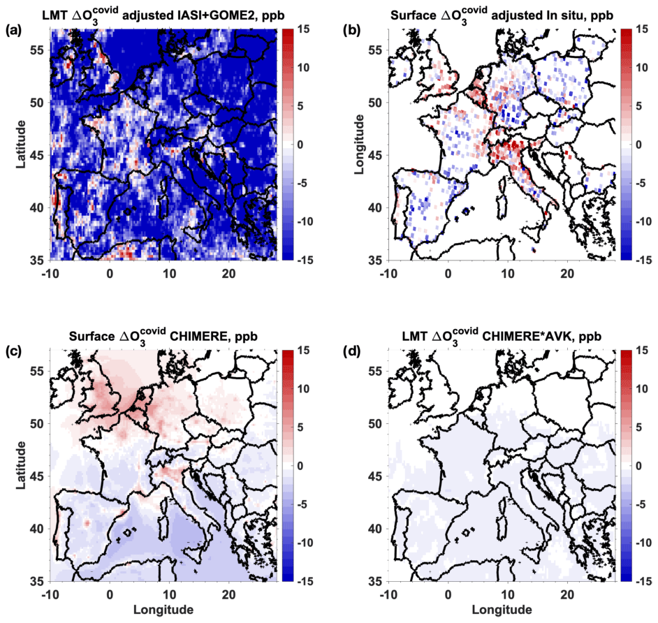
Figure 5Changes in ozone pollution (ppb) associated with the pandemic lockdown in 1–15 April 2020, derived from adjusted observations (using Eq. 1) for avoiding the influence of meteorological conditions at (a) the lowermost troposphere (LMT, < 3 km a.s.l.) retrieved with the IASI+GOME2 multispectral satellite approach and the surface, (b) measured by in situ sensors and simulated by the CHIMERE model (c) at the surface and (d) at the LMT smoothed by IASI+GOME2 averaging kernels.
3.3 Impact of COVID19 lockdown of spring 2020 in ozone pollution
Figure 3c shows net changes of ozone pollution only associated with the pandemic lockdown, which are derived from in situ measurements after subtracting the influence of meteorological conditions (using Eq. 1). In this case, it is expressed in terms of surface MDA8 concentrations during the month of April for comparison with previous studies. We observe an overall qualitative and quantitative consistency of the lockdown impact on ozone pollution estimated here (Fig. 3c) and those depicted by Ordóñez et al. (2020) and Souri et al. (2021). In the three estimates excluding meteorological effects, a net enhancement of surface ozone is seen across a region extending from southern England, Benelux, northeastern France/southwestern Germany, and northern Italy. Our estimate of the ozone enhancements over these regions (∼ 3 % in central Europe and ∼ 20 % over northern Italy) is similar to that estimated by Ordóñez et al. (2020) and Souri et al. (2021), ranging from ∼ 3 % to ∼ 8 % (according to Figs. 1 and 11, respectively, of these papers). On the other hand, net reductions of ozone concentrations are derived over southwestern and northeastern Europe of −7 % and −8 %, respectively (see Table 5). Over these regions, Ordóñez et al. (2020) roughly estimate a reduction −2 % to −7 %, whereas these values are near zero for the model-derived values from Souri et al. (2021).
Figure 5 presents lockdown-associated changes of ozone concentrations derived from IASI+GOME2 satellite retrievals, in situ measurements, and the CHIMERE model. The satellite-derived estimate of lowermost tropospheric ozone changes during 1–15 April 2020 (Fig. 7a) is clearly consistent with that derived from surface in situ measurements (Fig. 7b), both adjusted for avoiding the effects of meteorological conditions. The location of the positive and negative anomalies of ozone satellite retrievals is like that of total changes between 2020 and 2019 (Fig. 1a). Although, as for surface concentrations, the satellite-derived amplitude of the ozone enhancements linked to the lockdown over central Europe is clearly less pronounced than the total changes. Clear lockdown-derived enhancements of LMT ozone retrievals are seen over the Rhone Valley (reaching the Mediterranean), northern and eastern France, the Po Valley, and eastern England.
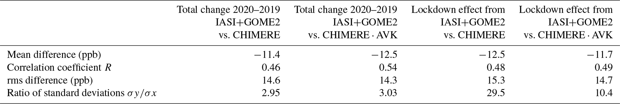
Table 3Same as Table 2 but comparing CHIMERE simulations with respect to the IASI+GOME2 lowermost tropospheric ozone retrievals. All CHIMERE model simulations correspond to LMT ozone columns coincident with IASI+GOME2 retrievals on a daily basis. The indication “⋅ AVK” is used when smoothing by the averaging kernels of IASI+GOME2.
Satellite data offer an extended geographical coverage with respect to surface in situ measurements. We observe a clear continuity in the ozone anomaly patterns in countries only partially or not sampled by in situ sensors, such as those of eastern Europe (from Latvia to Greece, with reductions of roughly −13 ppb) and other regions such as the Check republic, Austria, southern France, southern Italy, parts of Spain, and over the oceans. IASI+GOME2 depicts clear net reductions in ozone concentrations in 2020 south of the Mediterranean and part of the Atlantic west of France (respectively −11 and −8 ppb) and more important decreases over the North Sea (−21 ppb).
Model-only estimations of the impact of the pandemic lockdown on ozone pollution at the surface (Fig. 5c) show qualitative similarities and differences with respect to those using observations. Similar patterns of ozone enhancements up to ∼ 5 ppb are observed over eastern England, northern France, the Benelux, and northern Italy for observational methods and CHIMERE. This last one suggests a net ozone enhancement over the part of the Mediterranean Sea located south of France, which is associated with the reduction of shipping activities in this area and is also clearly observed by IASI+GOME2. On the other hand, the model simulates enhancements of ozone pollution over western England and the North Sea, where observations clearly suggest reductions. Over Germany and Poland, observations suggest the predominance of ozone reductions while CHIMERE indicates a moderate ozone enhancement (1–2 ppb). Simulated ozone reductions over the Atlantic, southern Mediterranean, and eastern Europe are clearly underestimated with respect to those observed by satellite. We can also notice that simulations overestimate the ozone enhancements over Germany and England and underestimate the ones over northern Italy, as compared to the two observational datasets. This can be partly attributed to the assumed homogenization of the lockdown conditions for these countries, whereas actual restrictions in Germany and England were less strict than in Italy.
On the other hand, we notice clear differences in the simulated changes associated with the pandemic lockdown for model-derived concentrations integrated up to 3 km of altitude (LMT) and also when smoothing with IASI+GOME2 averaging kernels (Fig. 5d). In these two last cases (see Table 3), CHIMERE only simulates a weak reduction of ozone over all of Europe and ozone enhancements become negligible. The range of variability of simulated concentrations decreases by more than a factor of 10, although the correlation with respect to IASI+GOME2 data remains fair (around ∼ 0.5). This suggests a clear underestimation of the amplitude of the effect of the pandemic lockdown simulated at atmospheric layers above the surface and within the LMT (< 3 km) as compared to IASI+GOME2 satellite observations.
A fair qualitative consistency is observed between observations (in situ and satellite) and CHIMERE datasets with respect to the regions of ozone enhancements and reductions associated with the pandemic lockdown conditions. Ozone increased over more urbanized regions with large NOx emissions, such as central northern Europe and the Po Valley, and mainly decreased far from NOx hotspots where night-time titration plays a less important role in the surface ozone daily balance. The significant model/observation difference over eastern Germany and Poland might be linked to the difficulty to accurately simulate neutral chemical regimes. There, an accurate simulation of competing terms of ozone production and sinks requires a larger precision of the emission inventories and other factors affecting the abundance of active chemical species.
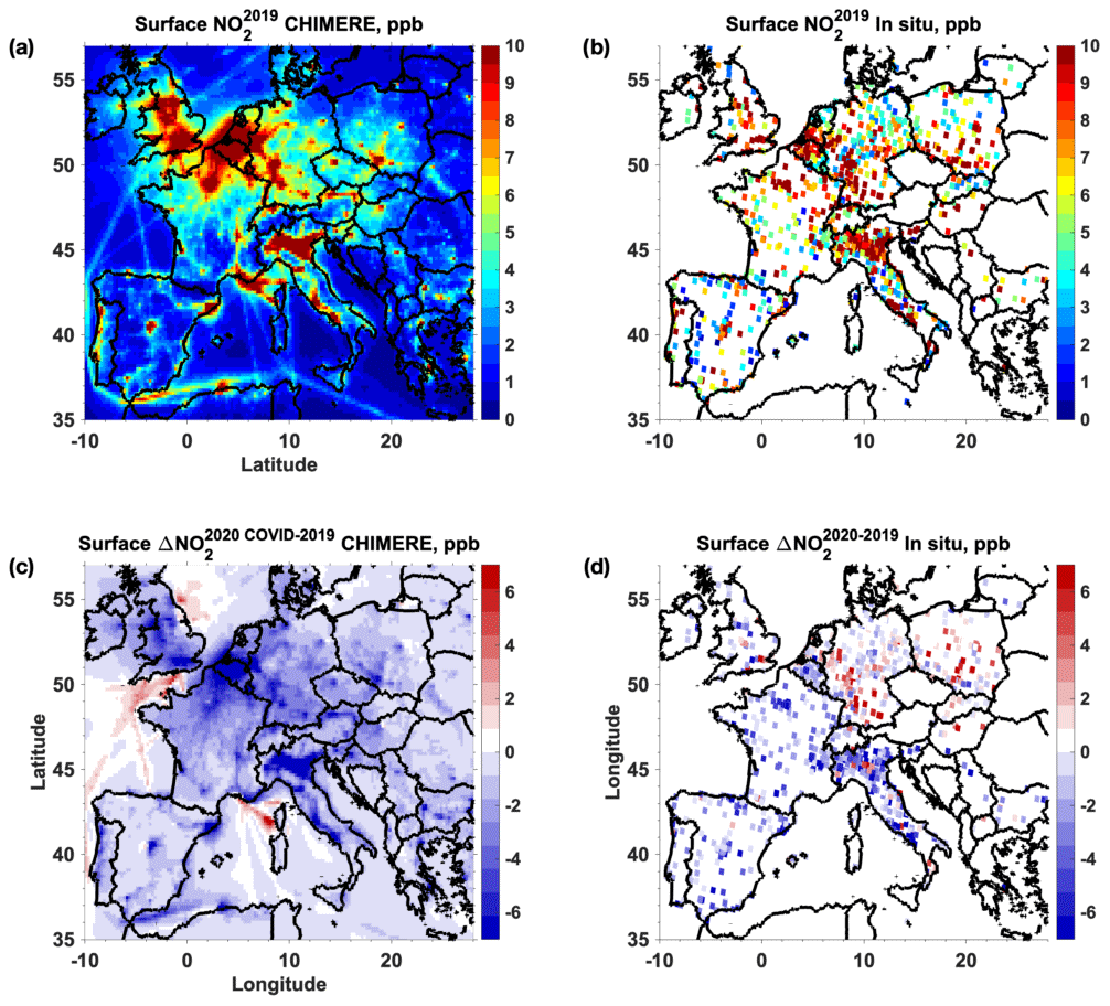
Figure 6Surface NO2 concentrations (ppb) averaged over the period 1–15 April 2019 (a) simulated by the CHIMERE and (b) measured by in situ sensors. Panels (c) and (d) are the same as panels (a) and (b), respectively, but for changes between 1–15 April 2020 with respect to the same period in 2019.
Table 4Changes of daily averages of surface ozone concentrations between 1–15 April 2020 and the same period in 2019, for four target regions in Europe (rectangles in Fig. 3a), derived from surface in situ measurements. Total, meteorological, and lockdown-associated changes are considered in mixing ratio units (ppb). Values after ± indicate 1 standard deviation.
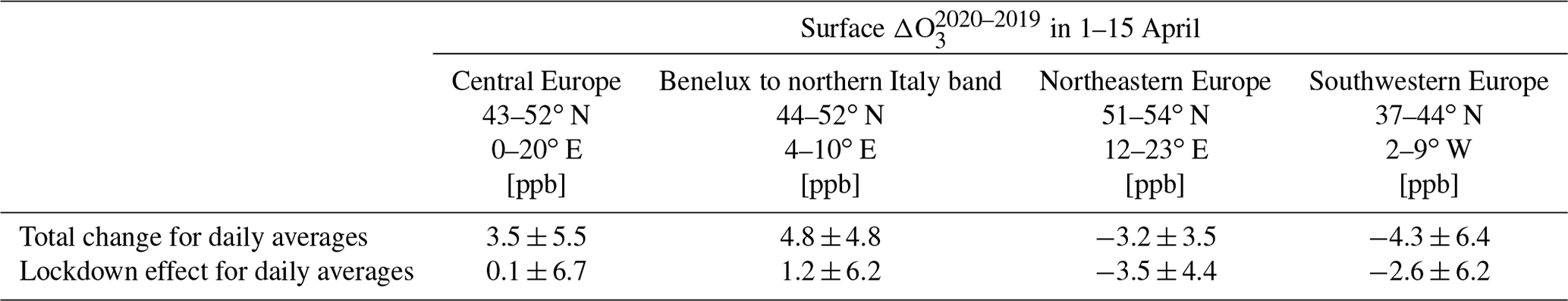
Table 5Same as Table 4 but for changes of MDA8 surface ozone concentrations averaged over the whole month of April and also percentage in italics.
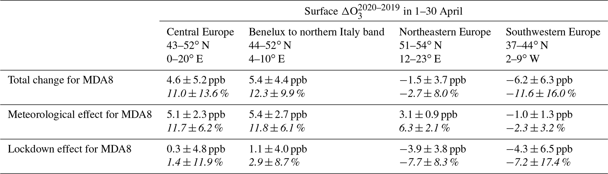
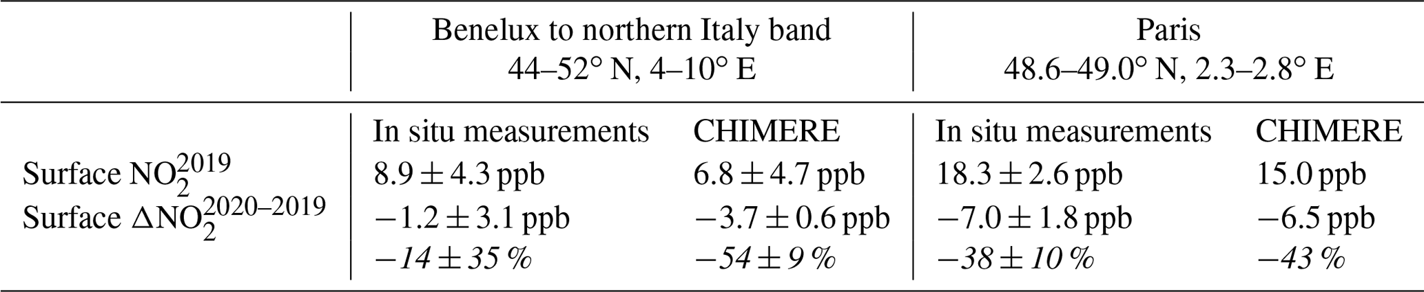
Table 6Comparison of nitrogen dioxide concentrations in the period 1–15 April 2019 and the changes between this period in 2020 with respect to 2019, for two target regions in Europe (rectangles in Fig. 3a), derived from surface in situ measurements and model simulations. Values after ± indicate 1 standard deviation and italics show percentage changes. Due to lack of representativity, model standard deviation within the Paris sector is not given.
Significant differences are seen in the amplitudes of the positive and negative anomalies of ozone pollution in spring 2020. On the one hand, in situ and satellite observations agree in terms of the total range of changes of ozone (both between 2020 and 2019 and adjusted for meteorological effects) of about ∼ 25 ppb between maximum positive and minimum negative anomalies over land, with satellite data shifted by ∼ 8 ppb towards smaller values (which can partly be linked to the altitude of sensitivity of these retrievals). On the other hand, CHIMERE underestimates the amplitude of these changes in ozone pollution (with the largest range for variability of ∼ 12 ppb), with respect to observations. This limited variability of ozone with respect to observations is also found for the chemistry-transport model of Souri et al. (2021) that uses adjusted European emissions of NOx and VOC with respect to satellite data. Particularly, we notice underestimations of the absolute amplitude of negative anomalies which are seen over land and over ocean with respect to satellite data. This may be partly explained by the fact that the model only accounts for the changes in ozone concentrations and its precursors associated with the pandemic lockdown over Europe, but other changes at a global scale are not considered. Nevertheless, the observational study of Steinbrecht et al. (2021) suggests that these last ones correspond to a significant ozone reduction in the free troposphere across the whole Northern Hemisphere in spring and summer 2020 (−7 % or −4 ppb over the northern extratropics). We likely expect this large-scale ozone reduction to be more pronounced at the beginning of this period (e.g. beginning of April 2020) as it is a period with more generalized and severe lockdowns over Europe and North America, as well as the last part of the lockdown over China and some restrictive measures over South Korea and Japan. Moreover, the ozone reduction in spring/summer 2020 is more noticeable near the North Sea (Lerwick) than for the south of France (Haute Provence) near the Mediterranean, as observed with the IASI+GOME2 retrievals over these two oceanic regions (Figs. 1a and 7a).
The amplitude of the ozone anomalies associated with the pandemic lockdown simulated by CHIMERE is likely related to the abundance of ozone precursors (Fig. 6). In 2019, NO2 simulated concentrations are lower than those measured by in situ measurements over a large heterogenous area such as the Benelux to northern Italy band and for a megacity such as Paris (see Table 6). For all in situ stations, the mean biases and root-mean-squared differences of coincident NO2 concentrations simulated in 2019 are quite significant (respectively around −5 and 6 ppb). When comparing with in situ measurements of , the measured reduction over a horizontally homogenous hotspot such as Paris clearly matches CHIMERE. Inversely, it is overestimated (by a factor ∼ 4) in absolute values over a heterogenous large area (such as the Benelux to northern Italy band). Therefore, the agreement between simulated and measured clearly depends on the criteria and the horizontal homogeneity of the abundances over the area considered in the comparison.
The uncertainties in the simulated NO2 concentrations are partly linked to the inventories used by the model. The CHIMERE model used here is based on emission inventories estimated for 2010 (by HTAPv2.2, on a monthly basis). A sustained negative trend for NO2 concentrations observed over Europe between 2010 and 2017 (e.g. Pazminio et al., 2021) suggests a positive bias for this inventory. This trend is ∼ 30 % in France, slightly higher in Italy or Belgium, and smaller for other countries such as Germany and Poland (∼ 13 %; see EMEP database, https://www.ceip.at/webdab-emission-database/emissions-as-used-in-emep-models, last access: 1 April 2022).
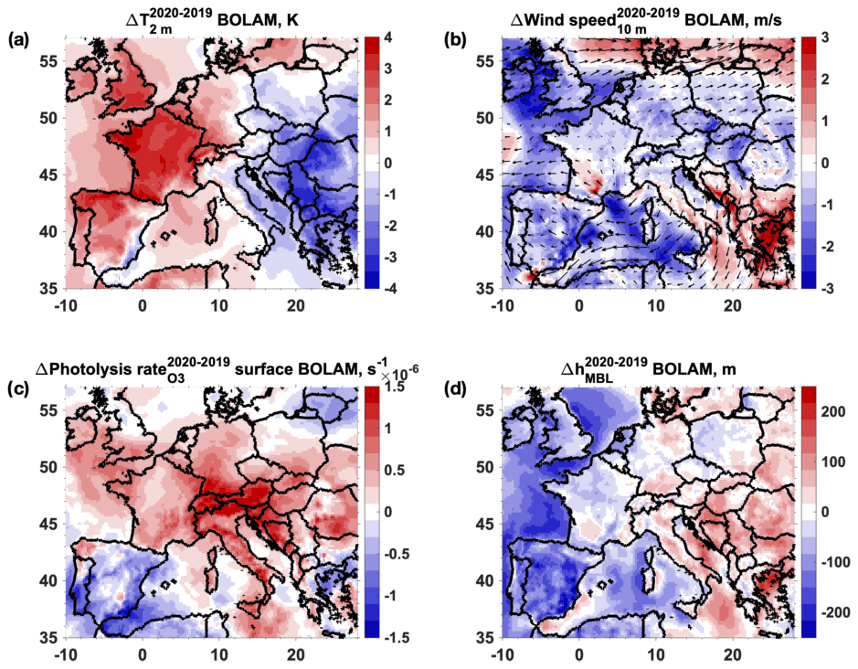
Figure 7Changes in (a) temperature at 2 m (K), (b) wind speeds (m s−1) and wind vectors, (c) ozone photolysis rates (s−1), and (d) height of the mixing boundary layer (m) averaged over the period 1–15 April 2020 with respect to the same period in 2019 from the meteorological fields used by CHIMERE.
Other factors significantly affecting simulated concentrations of ozone and its precursors are clearly linked to the meteorological fields used by the model. This is shown in terms of changes on 2020 with respect to 2019 of ozone photolysis rates, surface temperatures and winds, and mixing boundary layer heights used by CHIMERE (Fig. 7). Two distinct behaviours are clearly observed over the continent north of 44∘ N and over the Iberian Peninsula. North of 44∘ N, anticyclonic conditions prevailing in 2020 induced clearer sky conditions (thus enhancements of ozone photolysis rates), higher surface temperatures, and lower wind speeds, which clearly favour photochemical production of ozone. This explains the frank positive anomaly of surface ozone over this region visibly simulated by CHIMERE, accounting (Fig. 3a) or not (Fig. 4a) for the emission changes during the lockdown. Over the Iberian Peninsula, reduced ozone photolysis rates (Fig. 6a) associated with enhanced cloudiness in 2020 are likely at the origin of the meteorology-associated decrease in ozone concentrations (Fig. 3b). However, other meteorological conditions likely produce the opposite effect: enhanced surface temperatures and lower wind speeds in 2020 are expected to favour ozone production and shallower mixing boundary layers to inhibit turbulent vertical dilution of ozone, thus inducing a relative enhancement of surface ozone concentrations in 2020. These effects are expected to compensate between them, explaining the moderate reduction of ozone simulated by CHIMERE over this region (−2.4 % for the southwestern region in Table 5).
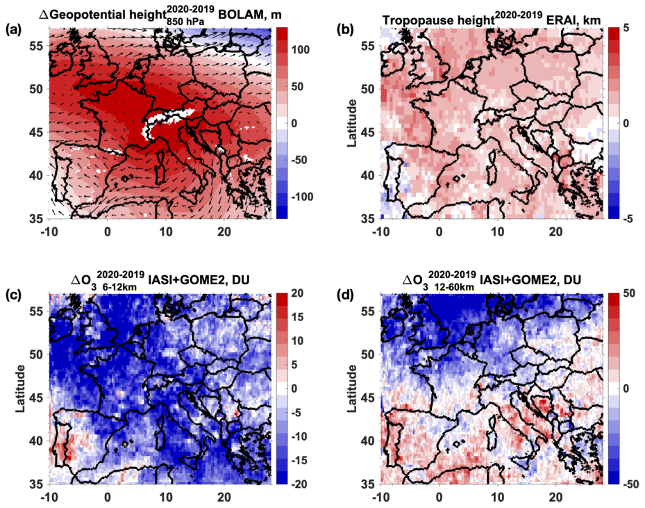
Figure 8Changes in (a) geopotential height (m) and wind vectors at 850 hPa from the BOLAM model, (b) tropopause heights (km) derived from vertical temperature profiles from ERA-Interim reanalyses from ECMWF, (c) ozone at 6–12 km of altitude (DU), and (d) ozone at 12–60 km of altitude (DU) retrieved from IASI+GOME2, averaged over the period 1–15 April 2020 with respect to the same period in 2019.
Furthermore, the variability of ozone at the free troposphere may also be a significant factor influencing near-surface ozone, depending on vertical mixing. The enhanced anticyclonic conditions in 2020 with respect to 2019 are particularly seen north of 44∘ N by increased geopotential heights and lower wind speeds at 850 hPa (Fig. 8a). This situation favours subsidence and thus vertical advection of air masses from the free troposphere down to the atmospheric boundary layer. This is less clearly noted over the Iberian Peninsula and the eastern Mediterranean, where a transition between lower and higher geopotential heights is seen (Fig. 8a). Ozone anomalies at the upper troposphere are depicted by IASI+GOME2 retrievals between 6 and 12 km in Fig. 8c. They mainly reveal an overall reduction of ozone concentrations in 2020 with respect to 2019, particularly over the North Sea and the central Mediterranean. This is probably related with the large-scale reduction of free tropospheric ozone in 2020 observed by Steinbrecht et al. (2021), mainly related with the lockdown-associated drop of precursor emissions over the Northern Hemisphere. Downward mixing of these ozone-poorer air masses probably contributes to the large-scale reduction of ozone observed at the LMT by IASI+GOME2 and its negative shift with respect to surface concentrations (Figs. 1 and 2a). Indeed, the only geographically coincident patterns observed both at the LMT and the upper troposphere are the ozone reductions of ozone over the Mediterranean and the North Sea.
At the upper troposphere, a near-zero variation is observed over northeastern Europe and an ozone enhancement over the western Iberian Peninsula (Fig. 8c). This last one is probably associated with coincident lower tropopause heights (Fig. 8b) and thus with a relatively larger contribution of stratospheric ozone. Over the North Sea, the reduction of upper tropospheric ozone at 6–12 km of altitude is strengthened by a depletion of stratospheric ozone occurring in 2020 (see in Fig. 8d as ozone anomalies with respect to 2019).
We have presented a comprehensive analysis using in situ and satellite measurements of ozone as well as chemistry-transport modelling tools of the changes in ozone pollution over Europe associated with the COVID-19 pandemic lockdown of springtime 2020. To the authors' knowledge, this is the first time that satellite direct observations of lowermost tropospheric ozone are used in such a multi-data analysis. While satellite observations of ozone show a fairly good agreement with respect to in situ surface measurements of ozone across Europe in the regions where both are available, only satellite data provide full horizontal coverage both over land and ocean (at 0.25∘ × 0.25∘ horizontal resolution). The observations quantify the changes of ozone pollution in 1–15 April 2020 with respect to the same period the previous year, thus the 15 d period when the lockdown measures modified the most anthropogenic activities over the continent.
An additional original aspect in the present analysis is the adjustment of both in situ and satellite observations for estimating the impact of the pandemic lockdown on ozone pollution, using measurements from 2020 and 2019. This adjustment is derived from the chemistry-transport model CHIMERE using the meteorological conditions of each year but the same standard (business-as-usual) anthropogenic emissions. This method relies on the model accuracy in standard conditions, and it neglects possible feedbacks between meteorological conditions and photochemical regimes. The influence of biogenic emissions is accounted for by the method, as these sources are derived according to the meteorological conditions. The adjustment can be directly applied to both in situ and satellite data, with good consistency with respect to other independent approaches used for the same kind of adjustment of surface in situ data (Ordóñez et al., 2020) or using integrated process rates derived from a chemical transport model (Souri et al., 2021).
The satellite and in situ observational estimates of the changes in ozone pollution associated with the pandemic lockdown show a significant enhancement of ozone in the VOC-limited regions of central and northern Europe and the Po Valley, as pointed out previously by models and in situ surface data (e.g. Menut et al., 2020; Ordóñez et al., 2020; Souri et al., 2021). This effect overlaps with a large-scale reduction of ozone over the whole continent (seen in the free troposphere by ozone sondes, Steinbrecht et al., 2021), which is clearly evidenced over the ocean (Atlantic, North and Mediterranean seas).
We compare these observation-based estimations with model-only estimates derived by changing emissions according to the reductions in anthropogenic activities estimated for the lockdown period. The model shows similar regional patterns of ozone enhancements and reductions linked to the lockdown, except for regions with neutral photochemical regimes (such as eastern Germany and Poland). However, it underestimates the amplitude of the positive and negative anomalies. Furthermore, the model does not simulate the ozone decrease observed at a large hemispheric scale or the stratospheric influence, as the simulation domain covers Europe and the troposphere. Sensitivity studies changing the emission inventory and meteorological conditions of the model highlight a particular sensitivity to vertical mixing within the lower atmospheric layers as a key factor influencing the amplitude of the ozone anomalies, as well as the emission inventories used for standard and lockdown conditions. The differences between simulations and observations highlight the complexity to simulate the effect of the changes in ozone concentrations due to changes in anthropogenic emissions, as occurred during the lockdown.
The IASI+GOME2 ozone dataset derived from MetOp-B global measurements in near real time is publicly available at the AERIS French national data centre. It can be accessed through the AERIS IASI portal on the permanent web page https://iasi.aeris-data.fr (IASI Portal, 2022a). The data policy is detailed in https://iasi.aeris-data.fr/data-use-policy/ (IASI Portal, 2022b). Additional IASI+GOME2 data (e.g. from other MetOp satellites) can be provided upon request to the principal investigator of the satellite data: Juan Cuesta, LISA/UPEC, cuesta@lisa.ipsl.fr.
The supplement related to this article is available online at: https://doi.org/10.5194/acp-22-4471-2022-supplement.
JC wrote the main part of the manuscript, analysed most the datasets, and provided IASI+GOME2 satellite data from multiple platforms. LC and BB performed CHIMERE model simulations and contributed to the analysis and writing of the manuscript. MB, GS, LM, and GD contributed to the analysis of the datasets and the text of the manuscript. GS has also collected the in situ data and provided it for the analysis. ME supported the processing of the satellite dataset. TL performed meteorological simulations and provided them for the CHIMERE model.
The contact author has declared that neither they nor their co-author has any competing interests.
Publisher's note: Copernicus Publications remains neutral with regard to jurisdictional claims in published maps and institutional affiliations.
This article is part of the special issue “Quantifying the impacts of stay-at-home policies on atmospheric composition and properties of aerosol and clouds over the European regions using ACTRIS related observations (ACP/AMT inter-journal SI)”. It is not associated with a conference.
Authors are grateful for the financial support of Centre National des Etudes Spatiales (CNES, the French Space Agency) via the SURVEYPOLLUTION project from TOSCA (Terre Ocean Surface Continentale Atmosphère), the Université Paris Est Créteil (UPEC), and the Centre National des Recherches Scientifiques–Institut National des Sciences de l'Univers (CNRS-INSU), for helping in achieving this research work and its publication.
We warmly acknowledge the French atmospheric data centre AERIS (https://www.aeris-data.fr, last access: 1 April 2022) for supporting the production of IASI+GOME2, the support of CNRS-INSU for the national communitarian code CHIMERE, data access and computing resources provided by the ESPRI IPSL mesocentre (https://mesocentre.ipsl.fr/, last access: 1 April 2022), the European Air Quality e-Reporting for in situ surface measurements of ozone and nitrogen dioxide, EUMETSAT for GOME-2 level 1 data (provided by the NOAA CLASS data portal), Copernicus Atmosphere Monitoring Service (CAMS) for the revised inventory of anthropogenic emissions during the COVID-19 lockdown in Europe, and Apple transport data. IASI is a joint mission of EUMETSAT and CNES. We thank the Institut für Meteorologie und Klimaforschung (Germany) and RT Solutions (USA) for licenses to use, respectively, the KOPRA and VLIDORT radiative transfer models. We also thank Zhaonan Cai from the Chinese Academy of Sciences (China) and Xiong Liu from the Harvard-Smithsonian Center for Astrophysics (USA) for their help to produce IASI+GOME2 data. The Programme National de Télédétection Atmosphérique (PNTS) and the Agence Nationale de la Recherche (ANR) also contributed in supporting the development of the IASI+GOME2 satellite product.
This research has been supported by the Centre National d'Etudes Spatiales (SURVEYPOLLUTION TOSCA project).
This paper was edited by Frank Dentener and reviewed by two anonymous referees.
Alfaro, S. C. and Gomes, L.: Modeling mineral aerosol production by wind erosion: emission intensities and aerosol size distribution in source areas, J. Geophys. Res., 106, 18075–18084, https://doi.org/10.1029/2000JD900339, 2001.
Barré, J., Petetin, H., Colette, A., Guevara, M., Peuch, V.-H., Rouil, L., Engelen, R., Inness, A., Flemming, J., Pérez García-Pando, C., Bowdalo, D., Meleux, F., Geels, C., Christensen, J. H., Gauss, M., Benedictow, A., Tsyro, S., Friese, E., Struzewska, J., Kaminski, J. W., Douros, J., Timmermans, R., Robertson, L., Adani, M., Jorba, O., Joly, M., and Kouznetsov, R.: Estimating lockdown-induced European NO2 changes using satellite and surface observations and air quality models, Atmos. Chem. Phys., 21, 7373–7394, https://doi.org/10.5194/acp-21-7373-2021, 2021.
Bauwens, M., Compernolle, S., Stavrakou, T., Müller, J. F., Van Gent, J., Eskes, H., Levelt, P. F., van der A, R., Veefkind, J. P., Vlietinck, J., Yu, H., and Zehner, C.: Impact of coronavirus outbreak on NO2 pollution assessed using TROPOMI and OMI observations, Geophys. Res. Lett., 47, e2020GL087978, https://doi.org/10.1029/2020GL087978, 2020.
Beekmann, M. and Vautard, R.: A modelling study of photochemical regimes over Europe: robustness and variability, Atmos. Chem. Phys., 10, 10067–10084, https://doi.org/10.5194/acp-10-10067-2010, 2010.
Bessagnet, B., Pirovano, G., Mircea, M., Cuvelier, C., Aulinger, A., Calori, G., Ciarelli, G., Manders, A., Stern, R., Tsyro, S., García Vivanco, M., Thunis, P., Pay, M.-T., Colette, A., Couvidat, F., Meleux, F., Rouïl, L., Ung, A., Aksoyoglu, S., Baldasano, J. M., Bieser, J., Briganti, G., Cappelletti, A., D'Isidoro, M., Finardi, S., Kranenburg, R., Silibello, C., Carnevale, C., Aas, W., Dupont, J.-C., Fagerli, H., Gonzalez, L., Menut, L., Prévôt, A. S. H., Roberts, P., and White, L.: Presentation of the EURODELTA III intercomparison exercise – evaluation of the chemistry transport models' performance on criteria pollutants and joint analysis with meteorology, Atmos. Chem. Phys., 16, 12667–12701, https://doi.org/10.5194/acp-16-12667-2016, 2016.
Bouarar, I., Gaubert, B., Brasseur, G. P., Steinbrecht, W., Doumbia, T., Tilmes, S., Liu, Y., Stavrakou, T., Deroubaix, A., Darras, S., Granier, C., Lacey, F., Müller, J.-F., Shi, X., Elguindi, N., and Wang, T.: Ozone anomalies in the free troposphere during the COVID-19 pandemic, Geophys. Res. Lett., 48, e2021GL094204, https://doi.org/10.1029/2021GL094204, 2021.
Buzzi, A., Tartaglione, N., and Malguzzi, P.: Numerical simulations of the 1994 Piedmont flood: Role of orography and moist processes, Mon. Weather Rev., 126, 2369–2383, https://doi.org/10.1175/1520-0493(1998)126<2369:NSOTPF>2.0.CO;2, 1998.
Clerbaux, C., Boynard, A., Clarisse, L., George, M., Hadji-Lazaro, J., Herbin, H., Hurtmans, D., Pommier, M., Razavi, A., Turquety, S., Wespes, C., and Coheur, P.-F.: Monitoring of atmospheric composition using the thermal infrared IASI/MetOp sounder, Atmos. Chem. Phys., 9, 6041–6054, https://doi.org/10.5194/acp-9-6041-2009, 2009.
Cuesta, J., Eremenko, M., Liu, X., Dufour, G., Cai, Z., Höpfner, M., von Clarmann, T., Sellitto, P., Foret, G., Gaubert, B., Beekmann, M., Orphal, J., Chance, K., Spurr, R., and Flaud, J.-M.: Satellite observation of lowermost tropospheric ozone by multispectral synergism of IASI thermal infrared and GOME-2 ultraviolet measurements over Europe, Atmos. Chem. Phys., 13, 9675–9693, https://doi.org/10.5194/acp-13-9675-2013, 2013.
Cuesta, J., Kanaya, Y., Takigawa, M., Dufour, G., Eremenko, M., Foret, G., Miyazaki, K., and Beekmann, M.: Transboundary ozone pollution across East Asia: daily evolution and photochemical production analysed by IASI+GOME2 multispectral satellite observations and models, Atmos. Chem. Phys., 18, 9499–9525, https://doi.org/10.5194/acp-18-9499-2018, 2018.
Deroubaix, A., Brasseur, G., Gaubert, B., Labuhn, I., Menut, L., Siour, G., and Tuccella, P.: Response of surface ozone concentration to emission reduction and meteorology during the COVID-19 lockdown in Europe, Meteorol. Appl., 28, 12 pp., https://doi.org/10.1002/met.1990, 2021.
Gaubert, B., Bouarar, I., Doumbia, T., Liu, Y., Stavrakou, T., Deroubaix, A., Darras, S., Elguindi, N., Granier, C., Lacey, F., Müller, J.-F., Shi, X., Tilmes, S., Wang, T., and Brasseur, G. P.: Global changes in secondary atmospheric pollutants during the 2020 COVID-19 pandemic, J. Geophys. Res.. Atmos., 126, e2020JD034213, https://doi.org/10.1029/2020JD034213, 2021.
Giani, P., Castruccio, S., Anav, A., Howard, D., Hu, W., and Crippa, P.: Short-term and long-term health impacts of air pollution reductions from COVID-19 lockdowns in China and Europe: a modelling study, Lancet Planetary Health, 4, e474–e482, https://doi.org/10.1016/S2542-5196(20)30224-2, 2020.
Gkatzelis, G. I., Gilman, J. B., Brown, S. S., Eskes, H., Gomes, A. R., Lange, A. C., McDonald, B. C., Peischl, J., Petzold, A., Thompson, C. R., and Kiendler-Scharr, A.: The global impacts of COVID-19 lockdowns on urban air pollution: A critical review and recommendations, Elementa: Science of the Anthropocene, 9, 00176, https://doi.org/10.1525/elementa.2021.00176, 2021.
Guenther, A., Karl, T., Harley, P., Wiedinmyer, C., Palmer, P. I., and Geron, C.: Estimates of global terrestrial isoprene emissions using MEGAN (Model of Emissions of Gases and Aerosols from Nature), Atmos. Chem. Phys., 6, 3181–3210, https://doi.org/10.5194/acp-6-3181-2006, 2006.
Honoré, C., Rouïl, L., Vautard, R., Beekmann, M., Bessagnet, B., Dufour, A., Elichegaray, C., Flaud, J., Malherbe, L., Meleux, F., Menut, L., Martin, D., Peuch, A., Peuch, V., and Poisson, N.: Predictability of European air quality: the assessment of three years of operational forecasts and analyses by the PREV'AIR system, J. Geophys. Res., 113, D04301, https://doi.org/10.1029/2007JD008761, 2008.
IASI Portal: Atmospheric composition data products, https://iasi.aeris-data.fr (last access: 1 April 2022), 2022a.
IASI Portal: Data Use Policy, https://iasi.aeris-data.fr/data-use-policy/ (last access: 1 April 2022), 2022b.
Janssens-Maenhout, G., Crippa, M., Guizzardi, D., Dentener, F., Muntean, M., Pouliot, G., Keating, T., Zhang, Q., Kurokawa, J., Wankmüller, R., Denier van der Gon, H., Kuenen, J. J. P., Klimont, Z., Frost, G., Darras, S., Koffi, B., and Li, M.: HTAP_v2.2: a mosaic of regional and global emission grid maps for 2008 and 2010 to study hemispheric transport of air pollution, Atmos. Chem. Phys., 15, 11411–11432, https://doi.org/10.5194/acp-15-11411-2015, 2015.
Kalnay, E., Kanamitsu, M., Kistler, R., Collins, W., Deaven, D., Gandin, L., Iredell, M., Saha, S., White, G., Woollen, J., Zhu, Y., Chelliah, M., Ebisuzaki, W., Higgins, W., Janowiak, J., Mo, K., Ropelewski, C., Wang, J., Leetmaa, A., Reynolds, R., Jenne, R., and Joseph, D.: The NCEP/NCAR 40-year reanalysis project, B. Am. Meteorol. Soc., 77, 437–471, https://doi.org/10.1175/1520-0477(1996)077<0437:TNYRP>2.0.CO;2, 1996
Le, T., Wang, Y., Liu, L., Yang, J., Yung, Y. L., Li, G., and Seinfeld, J. H.: Unexpected air pollution with marked emission reductions during the COVID-19 outbreak in China, Science, 369, 702–706, https://doi.org/10.1126/science.abb7431, 2020.
Mailler, S., Menut, L., Khvorostyanov, D., Valari, M., Couvidat, F., Siour, G., Turquety, S., Briant, R., Tuccella, P., Bessagnet, B., Colette, A., Létinois, L., Markakis, K., and Meleux, F.: CHIMERE-2017: from urban to hemispheric chemistry-transport modeling, Geosci. Model Dev., 10, 2397–2423, https://doi.org/10.5194/gmd-10-2397-2017, 2017.
Malguzzi, P., Buzzi, A., and Drofa, O.: The meteorological global model GLOBO at the ISAC-CNR of Italy assessment of 1.5 yr of experimental use for medium-range weather forecasts, Weather Forecast., 26, 1045–1055, 2011.
Marécal, V., Peuch, V.-H., Andersson, C., Andersson, S., Arteta, J., Beekmann, M., Benedictow, A., Bergström, R., Bessagnet, B., Cansado, A., Chéroux, F., Colette, A., Coman, A., Curier, R. L., Denier van der Gon, H. A. C., Drouin, A., Elbern, H., Emili, E., Engelen, R. J., Eskes, H. J., Foret, G., Friese, E., Gauss, M., Giannaros, C., Guth, J., Joly, M., Jaumouillé, E., Josse, B., Kadygrov, N., Kaiser, J. W., Krajsek, K., Kuenen, J., Kumar, U., Liora, N., Lopez, E., Malherbe, L., Martinez, I., Melas, D., Meleux, F., Menut, L., Moinat, P., Morales, T., Parmentier, J., Piacentini, A., Plu, M., Poupkou, A., Queguiner, S., Robertson, L., Rou”ıl, L., Schaap, M., Segers, A., Sofiev, M., Tarasson, L., Thomas, M., Timmermans, R., Valdebenito, 'A., van Velthoven, P., van Versendaal, R., Vira, J., and Ung, A.: A regional air quality forecasting system over Europe: the MACC-II daily ensemble production, Geosci. Model Dev., 8, 2777–2813, https://doi.org/10.5194/gmd-8-2777-2015, 2015.
Menut, L. and Bessagnet, B.: Atmospheric composition forecasting in Europe, Ann. Geophys., 28, 61–74, 2010.
Menut, L., Vautard, R., Flamant, C., Abonnel, C., Beekmann, M., Chazette, P., Flamant, P., Gombert, D., Guédalia, D., Lefebvre, M., Lossec .D.,.M., B., Mégie, G., Perros, P., Sicard, M., and Toupance, G.: Measurements and modelling of atmospheric pollution over the Paris area: an overview of the ESQUIF project, Ann. Geophys., 18, 1467–1481, 2000.
Menut, L., Coll, I., and Cautenet, S.: Impact of meteorological data resolution on the forecasted ozone concentrations during the ESCOMPTE IOP 2a and 2b, Atmos. Res., 74, 139–159, 2005a.
Menut, L., Schmechtig, C., and Marticorena, B.: Sensitivity of the sandblasting fluxes calculations to the soil size distribution accuracy, J. Atmos. Ocean. Tech., 22, 1875–1884, 2005b.
Menut, L., Bessagnet, B., Khvorostyanov, D., Beekmann, M., Blond, N., Colette, A., Coll, I., Curci, G., Foret, G., Hodzic, A., Mailler, S., Meleux, F., Monge, J.-L., Pison, I., Siour, G., Turquety, S., Valari, M., Vautard, R., and Vivanco, M. G.: CHIMERE 2013: a model for regional atmospheric composition modelling, Geosci. Model Dev., 6, 981–1028, https://doi.org/10.5194/gmd-6-981-2013, 2013.
Menut, L., Mailler, S., Siour, G., Bessagnet, B., Turquety, S., Rea, G., Briant, R., Mallet, M., Sciare, J., Formenti, P., and Meleux, F.: Ozone and aerosol tropospheric concentrations variability analyzed using the ADRIMED measurements and the WRF and CHIMERE models, Atmos. Chem. Phys., 15, 6159–6182, https://doi.org/10.5194/acp-15-6159-2015, 2015a.
Menut, L., Rea, G., Mailler, S., Khvorostyanov, D., and Turquety, S.: Aerosol forecast over the Mediterranean area during July 2013 (ADRIMED/CHARMEX), Atmos. Chem. Phys., 15, 7897–7911, https://doi.org/10.5194/acp-15-7897-2015, 2015b.
Menut, L., Bessagnet, B., Siour, G., Mailler, S., Pennel, R., and Cholakian, A.: Impact of lockdown measures to combat Covid-19 on air quality over western Europe, Sci. Total Environ., 741, 140426, https://doi.org/10.1016/j.scitotenv.2020.140426, 2020.
Mertens, M., Jöckel, P., Matthes, S., Nützel, M., Grewe, V., and Sausen, R.: COVID-19 induced lower-tropospheric ozone changes, Environ. Res. Lett., 16, 064005, https://doi.org/10.1088/1748-9326/abf191, 2021.
Miyazaki, K., Bowman, K., Sekiya, T., Takigawa, M., Neu, J. L., Sudo, K., Osterman, G., and Eskes, H.: Global tropospheric ozone responses to reduced Nox emissions linked to the COVID-19 worldwide lockdowns, Science Advances, 7, eabf7460, https://doi.org/10.1126/sciadv.abf7460, 2021.
Monahan, E. C.: The ocean as a source of atmospheric particles, in: The Role of Air–Sea Exchange in Geochemical Cycling, Kluwer Academic Publishers, Dordrecht, Holland, 129–163, https://doi.org/10.1007/978-94-009-4738-2_6, 1986.
Muhammad, S., Long, X., and Salman, M.: COVID-19 pandemic and environmental pollution: A blessing in disguise?, Sci. Total Environ., 728, 138820, https://doi.org/10.1016/j.scitotenv.2020.138820, 2020.
Nussbaumer, C. M., Pozzer, A., Tadic, I., Röder, L., Obersteiner, F., Harder, H., Lelieveld, J., and Fischer, H.: Tropospheric ozone production and chemical regime analysis during the COVID-19 lockdown over Europe, Atmos. Chem. Phys. Discuss. [preprint], https://doi.org/10.5194/acp-2021-1028, in review, 2021.
Ordóñez, C., Garrido-Perez, J. M., and García-Herrera, R.: Early spring near-surface ozone in Europe during the COVID-19 shutdown: Meteorological effects outweigh emission changes, Sci. Total Environ., 747, 141322, https://doi.org/10.1016/j.scitotenv.2020.141322, 2020.
Pazmiño, A., Beekmann, M., Goutail, F., Ionov, D., Bazureau, A., Nunes-Pinharanda, M., Hauchecorne, A., and Godin-Beekmann, S.: Impact of the COVID-19 pandemic related to lockdown measures on tropospheric NO2 columns over Île-de-France, Atmos. Chem. Phys., 21, 18303–18317, https://doi.org/10.5194/acp-21-18303-2021, 2021.
Potts, D. A., Marais, E. A., Boesch, H., Pope, R. J., Lee, J., Drysdale, W., Chipperfield, M. P., Kerridge, B., Siddans, R., Moore, D. P., and Remedios, J.: Diagnosing air quality changes in the UK during the COVID-19 lockdown using TROPOMI and GEOS-Chem, Environ. Res. Lett., 16, 054031, https://doi.org/10.1088/1748-9326/abde5d, 2021.
Rouïl, L., Honoré, C., Vautard, R., Beekmann, M., Bessagnet, B., Malherbe, L., Meleux, F., Dufour, A., Elichegaray, C., Flaud, J., Menut, L., Martin, D., Peuch, A., Peuch, V., and Poisson, N.: PREV'AIR: an operational forecasting and mapping system for air quality in Europe, B. Am. Meteorol. Soc., 90, 73–83, https://doi.org/10.1175/2008BAMS2390.1, 2009.
Shi, X. and Brasseur, G. P.: The response in air quality to the reduction of Chinese economic activities during the COVID-19 outbreak,. Geophys. Res. Lett., 47, e2020GL088070, https://doi.org/10.1029/2020GL088070, 2020.
Sicard, P., De Marco, A., Agathokleous, E., Feng, Z., Xu, X., Paoletti, E., Diéguez Rodriguez, J. J., and Calatayud, V.: Amplified ozone pollution in cities during the COVID-19 lockdown, Sci. Total Environ., 735, 139542, https://doi.org/10.1016/j.scitotenv.2020.139542, 2020.
Souri, A. H., Chance, K., Bak, J., Nowlan, C. R., González Abad, G., Jung, Y., Wong, D. C., Mao, J., and Liu, X.: Unraveling pathways of elevated ozone induced by the 2020 lockdown in Europe by an observationally constrained regional model using TROPOMI, Atmos. Chem. Phys., 21, 18227–18245, https://doi.org/10.5194/acp-21-18227-2021, 2021.
Steinbrecht, W., Kubistin, D., Plass-Dülmer, C., Davies, J., Tarasick, D. W., Gathen, P. V. D., Deckelmann, H., Jepsen, N., Kivi, R., Lyall, N., Palm, M., Notholt, J., Kois, B., Oelsner, P., Allaart, M., Piters, A., Gill, M., Malderen, R. V., Delcloo, A. W., Sussmann, R., Mahieu, E., Servais, C., Romanens, G., Stübi, R., Ancellet, G., Godin-Beekmann, S., Yamanouchi, S., Strong, K., Johnson, B., Cullis, P., Petropavlovskikh, I., Hannigan, J. W., Hernandez, J.-L., Rodriguez, A. D., Nakano, T., Chouza, F., Leblanc, T., Torres, C., Garcia, O., Röhling, A. N., Schneider, M., Blumenstock, T., Tully, M., Paton-Walsh, C., Jones, N., Querel, R., Strahan, S., Stauffer, R. M., Thompson, A. M., Inness, A., Engelen, R., Chang, K.-L., and Cooper, O. R.: COVID-19 crisis reduces free tropospheric ozone across the Northern Hemisphere, Geophys. Res. Lett., 48, e2020GL091987, https://doi.org/10.1029/2020GL091987, 2021.
Szopa S., Foret, G., Menut, L., and Cozic, A.: Impact of large scale circulation on European summer surface ozone: consequences for modeling, Atmos. Environ., 43, 1189–1195, https://doi.org/10.1016/j.atmosenv.2008.10.039, 2009.
Thunis, P., Clappier, A., Beekmann, M., Putaud, J. P., Cuvelier, C., Madrazo, J., and de Meij, A.: Non-linear response of PM2.5 to changes in NOx and NH3 emissions in the Po basin (Italy): consequences for air quality plans, Atmos. Chem. Phys., 21, 9309–9327, https://doi.org/10.5194/acp-21-9309-2021, 2021.
Vautard, R., Beekmann, M., and Menut, L.: Applications of adjoint modelling in atmospheric chemistry: sensitivity and inverse modelling, Environ. Model. Softw., 15, 703–709, 2000.
Vivanco, M., Bessagnet, B., Cuvelier, C., Theobald, M., Tsyro, S., Pirovano, G., Aulinger, A., Bieser, J., Calori, G., Ciarelli, G., Manders, A., Mircea, M., Aksoyoglu, S., Briganti, G., Cappelletti, A., Colette, A., Couvidat, F., D'Isidoro, M., Kranenburg, R., Meleux, F., Menut, L., Pay, M., Rouil, L., Silibello, C., Thunis, P., and Ung, A.: Joint analysis of deposition fluxes and atmospheric concentrations of inorganic nitrogen and sulphur compounds predicted by six chemistry transport models in the frame of the EURODELTAIII project, Atmos. Environ., 151, 152–175, https://doi.org/10.1016/j.atmosenv.2016.11.042, 2017.
Wilson, R. C., Fleming, Z. L., Monks, P. S., Clain, G., Henne, S., Konovalov, I. B., Szopa, S., and Menut, L.: Have primary emission reduction measures reduced ozone across Europe? An analysis of European rural background ozone trends 1996–2005, Atmos. Chem. Phys., 12, 437–454, https://doi.org/10.5194/acp-12-437-2012, 2012.
Ziemke, J. R., Kramarova, N. A., Huang, L. K., Herman, J. R., Bhartia, P. K., and Wargan, K.: Evaluation and Validation of Tropospheric Ozone Hourly and Daily Maps Measured from EPIC, OMPS, OMI, and MLS Satellite Instruments, Presented at CEOS AC-VC 17 meeting https://ceos.org/document_management/Virtual_Constellations/AC-VC/Meetings/AC-VC-17/3.Wednesday-Ozone/3.04_ziemke_v1.ppt (last access: 1 April 2022), 2021.