


Introduction
On 11 March 2020 the World Health Organization (WHO) declared the novel coronavirus outbreak (severe acute respiratory syndrome-coronavirus-2 (SARS-CoV-2) causing coronavirus disease 2019 (COVID-19)) a pandemic [1] more than three months after the first cases of pneumonia were reported in Wuhan, China in December 2019 [1]. From Wuhan the virus rapidly spread globally, currently leading to tens of millions of confirmed cases and over a million deaths around the world. Although coronaviruses have a wide range of hosts and cause disease in many animals, SARS-CoV-2 is the seventh named member of the Coronaviridae known to infect humans [Reference Sun2]. An infected individual will start presenting symptoms an average of five days after exposure [Reference Rothan and Byrareddy3] but it has been reported that 42% of infected individuals remain asymptomatic [Reference Mizumoto4, Reference Nishiura5]. In early November 2020, 2.5% people officially diagnosed with COVID-19 had died [6] while treatment and vaccine options for COVID-19 were limited [Reference Cowling7]. A report from April 2020 noted 78 active vaccine projects, and some of the more recent results are quite promising with a number of vaccines being widely deployed in early 2021, although full worldwide distribution will likely still take several years [Reference Thanh Le8–Reference Ramasamy10]. Fortunately, aggressive contact tracing [11] and social isolation methods [Reference Cowling7, Reference Koo12, Reference Bavel13] as well as pharmaceutical interventions such as the steroid dexamethasone [14] and convalescent plasma [Reference Bloch15] have shown some efficacy against the disease. As the virus is transmitted mainly from person to person, prevention measures include social distancing, self-isolation, hand washing and use of masks. Strict measures of quarantine have been shown to be the currently most effective mitigation measures, reducing up to 78% of expected cases compared to no intervention [Reference Koo12]. Nevertheless, to evaluate the actual effectiveness of any mitigation measure it is necessary to accurately predict the expected number of cases in the absence of intervention as an accurate number will better inform decisions about relaxing the mitigation measures which can be both economically and politically costly.
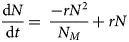
While there has been some early concern about the ability of SARS-CoV-2 to spread at an apparent near exponential rate [Reference Roosa16, Reference Ziff and Ziff17], limitations in available resources (i.e. susceptible population, sub-optimal mixing of infected and susceptible populations [Reference King18] etc.) will reduce the spread of any real (non-theoretical) disease to a logistic (sub-exponential) growth rate [Reference Tsoularis19]. Logistic growth produces a sigmoidal curve over time (Fig. 1) where the total number of cases (N) eventually (barring new births [Reference Cobey20]) asymptotically approaches the population carrying capacity (NM), which for viral epidemics is analogous to the fraction of the population that will be infected before ‘herd immunity’ is achieved [Reference Anderson and May21–Reference Ma23]. This is represented in derivative form by the generalised logistic function (Equation 1):

where α, β and γ are the mathematical shape parameters that define the shape of the curve and r is the general rate term, analogous to the standard epidemiological parameter, R 0 [Reference Fine, Eames and Heymann22, Reference Liu24]. For a logistic curve where α = ½ and β = γ = 0, one gets quadratic growth [Reference Brandenburg25] with N = (rt/2)2. For α = ½ and β = γ = 1, we have quadratic growth with saturation (Supplemental Appendix 1) while for α = β ≠γ = 1, this equation can be re-arranged to quadratic form (Equation 2) [Reference Tsoularis19] and integrated (Equation 3):

where N 0 represents the initial number of cases within the population. The shape parameters of logistic functions magnify the uncertainty in fitting these curves especially during the early part of the epidemic. These difficulties are further exacerbated by the additional uncertainty in estimation of R 0 for SARS-CoV-2, which is directly linked to the current uncertainty in the population carrying capacity NM. And while the basic logistic function gives rise to a symmetrical sigmoidal curve, asymmetrical curves such as the Gompertz growth function (Equation 4) [Reference Tjorve and Tjorve26, Reference Laird27]:
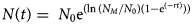
which emerges [Reference Tsoularis19] from Equation 1 for α = γ = 1, where r is replaced by β r and β approaches zero. For Gompertz growth, the rate of spread slows significantly after passing the mid-point resulting in long-tailed epidemics (Fig. 1).
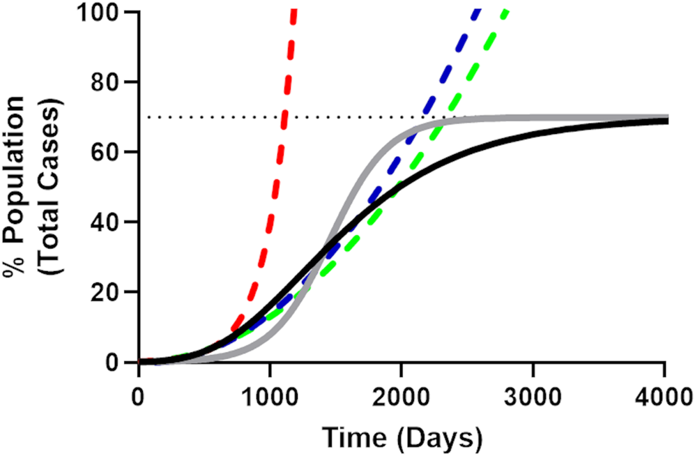
Fig. 1. Illustrative comparison of exponential, quadratic, generalised logistic and Gompertz growth curves. The Gompertz growth curve (Equation 4, solid black line) representing the progress of a theoretical epidemic for a disease with an arbitrarily chosen R 0 value of 3.4 (r = 0.045, N 0 = 1, NM = 70%, dotted line). The solid grey line is an equivalent logistic curve, note that while the midpoint for both logistic curves is the same, the Gompertz curve reaches the population carrying capacity more slowly, resulting in a long-tailed epidemic. The initial part of the Gompertz curve (including time points until 5% of the population has been infected) was fit to the simple exponential (red dashes), quadratic (blue dashes) and simple square (green dashes) models. It is apparent from these curves how quickly the exponential curve overestimates the rate of growth for the epidemic as compared to the quadratic and simple square fit curves and how the quadratic model more closely follows the Gompertz growth curve, evidenced by the smaller Sy.x value for the quadratic fit in Table 1.
Table 1. Average statistical fit parameters for the quadratic, simple square, simple exponential and Gompertz growth models for the early course of the epidemic in each country

a Because fit parameters were unable to be obtained for the Gompertz model for two countries, the statistical parameters were calculated from the remaining 26 countries (indicated by N = 26). The generalised logistic model failed to adequately determine fit parameters in every case so is not included in this table. The prediction error is the mean difference between the prediction for the final day of the curve and the actual total number of cases for that day in each country.
Traditionally, the number of cases that will occur in an epidemic like COVID-19 is modelled with an SEIR model (Susceptible, Exposed, Infected, Recovered/Removed), in which the total population is divided into four categories: susceptible – those who can be infected, exposed – those who are in the incubation period but not yet able to transmit the virus to others, infectious – those who are capable of spreading disease to the susceptible population and recovered/removed – those who have finished the disease course and are not susceptible to re-infection or have died. For a typical epidemic, the ability for infectious individuals to spread the disease is proportional to the fraction of the population in the susceptible category. ‘Herd immunity’ [Reference Anderson and May21, Reference Fine, Eames and Heymann22] and extinction of the epidemic occurs once a limiting fraction of the population has entered into the Recovered/Removed category [Reference Fine, Eames and Heymann22]. However, barriers to transmission, either natural [Reference Vora, Burke and Cummings28] or artificial (i.e. quarantines, vaccines) [Reference Fine, Eames and Heymann22] can extinguish the epidemic before the community is fully infected. Artificial barriers such as mandatory quarantining in China [Reference Kupferschmidt and Cohen29, Reference Maier and Brockmann30] or aggressive contact tracing in South Korea [11] seem to have largely stemmed the spread of SARS-CoV-2 during the early portion of the pandemic. Numerous political, social and material factors hamper the implementation of either of these responses in many other countries [Reference Bavel13], but it should be possible to find alternative approaches which can be equally effective. For an epidemic as serious as COVID-19, it behooves medical, scientific and policy experts to determine as rapidly as possible which community responses are effective and achievable within different populations. However, predictive underestimation will dampen response efforts while overestimation of the expected number of cases will make neutral or even harmful responses appear incorrectly to be effective when those overestimated cases fail to occur. Thus, accurate prospective predictions (i.e. before knowing the actual outcome) are preferable to retrospective analysis in which effectiveness is gauged after the results of the prescriptive actions are known [Reference Yang31, Reference Friedman32].
This study aimed to evaluate if a simple model was able to correctly fit the total number of confirmed cases and if that could be used to extrapolate to the total number of cases at a future date [Reference Ma23]. We found that fitting the case data from the early portion of the pandemic to a quadratic (parabolic) rate curve [Reference Brandenburg25] for the early days of the individual national epidemics was easy, efficient and able to accurately estimate the number of cases at future dates despite significant national variation in the start of the infection, mitigation response or economic condition.
Methods
Data on the number of COVID-19 cases was downloaded from the European Centre for Disease Prevention and Control (ECDC) on 1 June 2020 and 10 October 2020 [33]. Countries that had reported the highest numbers of cases in mid-March 2020 (and Russia) were chosen as the focus of our analysis to minimise statistical error due to small numbers (although we were able to get good fits to data in both Australia and Malaysia which had less than 5000 total cases before the effect of interventions had become obvious). The total number of cases for each country was calculated as a simple sum of that day plus all previous days including days before the start of the fitting curve. Days that were missing from the record were assigned values of zero. The early part of the curve was fit and statistical parameters were generated using Prism 8 (GraphPad) using the method of least squares as implemented in the non-linear regression module using the program standard centred second-order polynomial (quadratic), exponential growth and the Gompertz growth model as defined by Prism 8, and a simple user-defined simple square model (N = At 2 + C) where N is the total number of cases, A and C are the fitting constants and t is the number of days from the beginning of the epidemic curve. The beginning of the curve was defined manually from among the first days in which the number of cases began to increase regularly without interruption by any days with zero officially reported cases. Typically, this occurred when the country had reported less than 100 total cases. Model fitting used at least five days of data at a minimum. The specific starting fit day for each country is given in Figures 2 and 3. The early part of the curve was defined by manual examination looking for changes in the curve shape and later confirmed by R 2 values for the quadratic model (Fig. 2). Projections for the number of cases at the end of the fit were generated by fitting the total number of COVID-19 cases for each day starting with day 5 and then extrapolating the number of cases using the estimated model parameters to estimate the number of cases for the final day for which data were available at the time (1 June 2020) or to the last day before significant decrease in the R 2 value (R 2 < 0.95) for the quadratic fit. Fit parameters for the Gompertz growth model were not used for projections if the fit itself was ambiguous. The incidence (number of new cases per day) was calculated by subtracting the total number of cases on the previous day, examined over several day intervals. Estimates of the total future accuracy of the four models was estimated by predicting forward by 60 days for each of the four models when compared to the actual reported number of total cases using the fit parameters calculated as above (in many cases beyond the original final day of 1 June 2020). A prediction was judged to be successful if the total number of cases was within the range calculated from the 95% confidence interval (CI) fit values. Successful predictions were given a scoring reward of one point divided by half the width of the prediction interval in cases, while unsuccessful predictions were given zero points (Fig. 3). Instances of when the Gompertz model failed to fit all the parameters for the estimate of total accuracy were given a score of zero for that day. The bias was calculated as the amount of over or under prediction compared to the actual number of cases. The width was calculated as the difference between the limits of the 95% CI and normalised to the actual number of cases for that day.
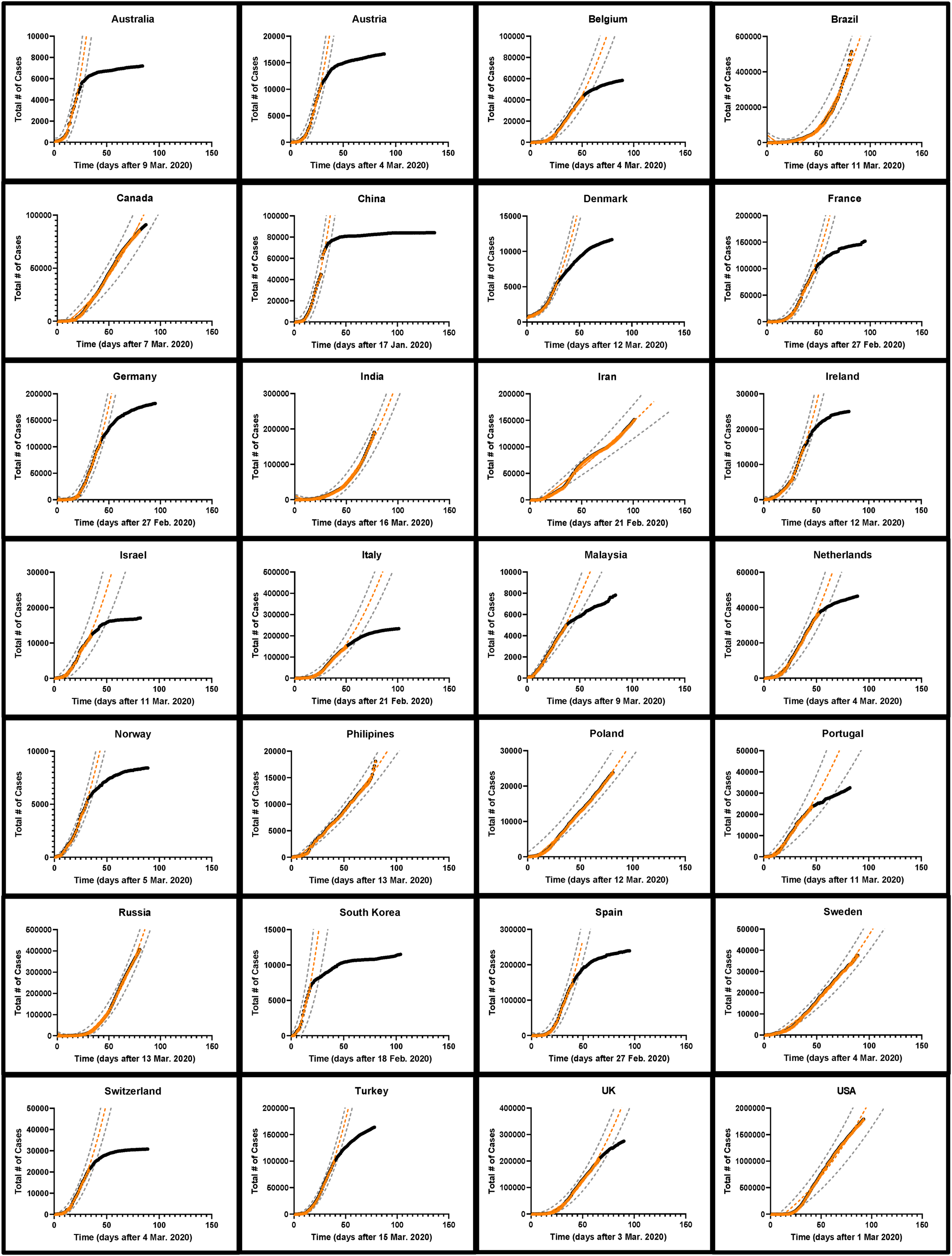
Fig. 2. The development of COVID-19 cases over time in 28 nations. The total number of cases as of 1 June 2020 is indicated by black circles while the early part of the curve is indicated by orange triangles. A quadratic fit curve based on the early part of the curve extrapolated into the future is shown as an orange dashed line. The first day of each fit curve is listed for each country. The black circles are obscured in those countries which had not begun to effectively reduce SARS-CoV-2 spread by 1 June 2020. The range of possible values corresponding to the 95% confidence interval around the predicted number of cases is indicated with dashed grey lines [Reference Colilla58].
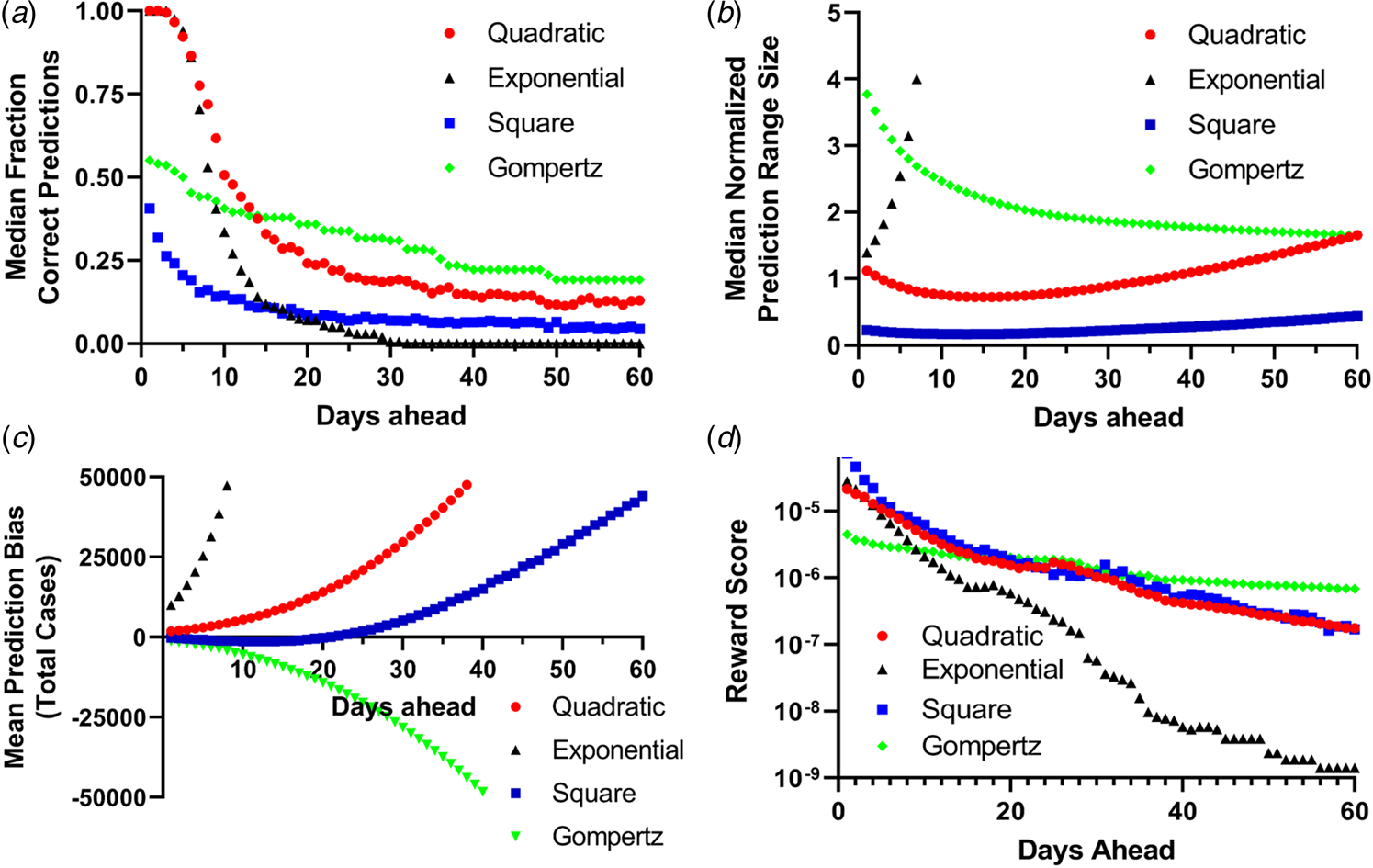
Fig. 3. Binary scoring of total future predictions from the four models. (a) Median success rate for the number of days in the future for every fit data point (the orange points in Fig. 2) for predictions within the 95% CI for the fit parameters. (b) Mean normalised width of the 95% CI predictions for all 28 countries for up to 60 days in advance. (c) Mean prediction bias among all 28 countries for all four models. (d) Reward score for all 28 countries for all four prediction methods.
Results
A simple exponential growth model is a poor fit for the SARS-CoV-2 pandemic
The cumulative number of confirmed cases for the early portion of the epidemic in each of 28 countries was plotted with time and several model equations were fit to the early part of the data before the mitigating effects from public health policies arrested disease spread. We expect that changes in the trajectory of the cumulative number of cases over time would indicate the efficacy of these mitigation effects. In total, 20 (71%) countries showed an obvious change in the curvature of the trajectory of the total number of cases by 1 June 2020 (Fig. 2). When the early portion of the data (with an unchanged trajectory) was examined for all 28 countries, the Gompertz growth model had the best statistical parameters (mean R 2 = 0.998 ± 0.0028, Table 1) although an overall fit could not be obtained for the data from two countries and many of the fit values for NM were unrealistic compared to national populations (e.g. China and India had fit NM values corresponding to 0.014 and 0.33% of their populations, respectively [33] (SI Table 1)). Fitting was also incomplete for the generalised logistic model for all 28 countries underlining the difficulty in applying this model. On the other hand, the simple models were able to robustly fit all the current data, with the quadratic (parabolic) model performing the best (mean R 2 = 0.992 ± 0.004) and the exponential model the worst (mean R 2 = 0.957 ± 0.022) (Table 1). In only three (11%) countries did the exponential model have the best overall R 2 value among the simple models. Furthermore, the trend of the overall superiority of the Gompertz model followed by the quadratic was observed in the sum of squares, AICc and the standard error of the estimate statistics. The sum of squares is smallest for the Gompertz model in 24 of the 28 countries (86%), while the quadratic model is the best of the remaining three models in 25 of the 28 countries (89%). The Gompertz model had the best AICc in 24 of the 28 countries (86%) and again the quadratic model was the best of the remaining three models in 22 of 28 countries (79%). This was also reflected in the average values of the AICc among all countries (Table 1). The mean standard error of the estimate (Sy.x, analogous to the root mean-squared error for fits of multiple parameters) value for the 28 countries was 1699 for the Gompertz model, 5613 for the quadratic model, 8572 for the simple square model and 11 257 for the exponential model (Table 1). Likewise, plots of the natural log of the total number of cases in the early parts of the epidemic (ln N) with time are significantly less linear (as determined by R 2) than equivalent plots of the square root of the total number of cases (N 1/2) (SI Table 2, SI Figs 1 and 2).
Quadratic growth models provide improved fits to the early portion of the epidemic courses
While logistic growth models have been widely used to model epidemics [Reference Tjorve and Tjorve26, Reference Liu, Tang and Xiao34, Reference Viboud, Simonsen and Chowell35], uncertainties in estimates of R 0 (and therefore the population carrying capacity NM) make modelling the epidemic difficult [Reference Liu24, Reference Liu, Tang and Xiao34]. (Fig. 4, Table 2, SI Table 3). For most countries, projection from the simple exponential model massively overpredicted the cumulative number of future cases. Projections generated more than 14 days prior to the final date suggested more than double the actual number of cases for 17 (61%) countries examined. In fact, for 15 (54%) countries, the exponential model gave at least one projection that differed from the eventual final day case number by a factor of greater than 10 000 fold, while the quadratic and simple square models made no final day overprediction by more than a factor of 3.3 and 2.1, respectively (i.e. using the first 10 days of data from Portugal projection using the exponential model projects 34 million cases while the quadratic, simple square and Gompertz growth models projects 24 957, 20 358 and 18 953 cases, respectively, while 23 683 total cases were actually observed on the final day. The total population of Portugal in 2018 was 10.3 million [33]). When using the quadratic fit model to project the number of new daily cases (incidence) [Reference King18, Reference Ma23], the actual number of cases for the final day was within the limits established by the 95% CI from the fit parameters was successfully predicted on average 63% of the time for all 28 countries when a 7-day prediction window was examined (Table 3).

Fig. 4. Comparison of the errors in final day prospective predictions for COVID-19 case numbers for different growth models for 28 countries for the simple exponential model (red triangles), the simple square model (green squares), the quadratic model (black circles), the Gompertz growth model (blue triangles) and the basic logistic growth model (purple diamonds). The first day of each fit curve is listed for each country. Note the log scale for the vertical axis which indicates the ratio of the predicted to observed number of cases. In each graph the fit values for each model using only data up to that day are used to predict the number of expected cases for the last day for which data are available (or the last day before significant curve deviation is observed, see Fig. 2). Days on which the fit was not statistically sound for the Gompertz model were omitted from the graph.
Table 2. Results of prospective predictions for total case load made using the various models for final day predictions
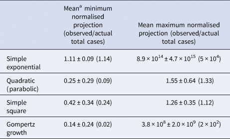
a All data given are mean results ± the sample standard error. Median values are given in parentheses.
Table 3. Fraction of successful predictions of the incidence of new cases of COVID-19 using the quadratic model. The incidence (number of new cases per day) was calculated by subtracting the total number of cases on the previous day

Results are given as the fraction of successful predictions. A prediction was judged to be successful if the total number of cases (actual) fell between the limit values of the prediction using the totals generated by the 95% CI from the fit parameters using the sum of predictions with 5, 7 and 12 day intervals calculated for all possible intervals for each country using the same days as from the regular quadratic model fits (Fig. 2).
Projections using the quadratic and simple square models much more closely matched the observed final day case numbers. Only in four (14%) countries did the quadratic model ever overpredict the final number of cases by more than a factor of 2, while the simple square model overpredicted by a factor of 2 or greater for only one (4%) country (SI Table 3). For the quadratic model, the mean maximum daily overprediction was a factor of 1.6-fold (median 1.3-fold), while for the simple square model the mean maximum daily overprediction was 1.3-fold (median 1.1-fold). Both of these models produced much more accurate projections than the simple exponential model (Table 2). We also estimated the total accuracy of these simple models by assigning a binary success/failure score to predictions up to 60 days in advance for each day of the originally fit data and examining the width and bias towards over and underprediction for each model [Reference Gneiting and Raftery36, Reference Funk37] as well as using a simple scoring metric (Fig. 3). Both the quadratic and exponential models made fairly accurate predictions up to 10 days in advance, although the quality of forecasts from the exponential model quickly deteriorates further into the future and this is more obvious when the scoring metric is applied. The exponential model also produces much larger ranges of predicitions within the 95% CI than the other models and quickly begins to significantly over predict the number of future total cases. Both the quadratic and exponential model tended to overpredict the number of future cases, while the simple square model tended to underpredict up to 10 days in advance but overpredict further into the future, while the Gompertz model generally underpredicted the total number of cases. Likewise, while all the models had a generalised expansion of their 95% CI prediction ranges more than 15 days in the future, this expansion was most significant for the exponential model.
Discussion
The start of the global SARS-CoV-2 pandemic has resulted in an unprecedented set of national responses. These responses have varied considerably from a strict lockdown in China [Reference Roosa16], to aggressive contact tracing in South Korea [Reference Oh38], to mandatory shelter in place restrictions in France [Reference Moatti39], to giving citizens information and allowing them more freedom to make choices as in Sweden [Reference Sjodin40] and to other countries which appeared to be considering attempts to accelerate their progress towards herd immunity [Reference Altmann, Douek and Boyton41, Reference Vogel42]. The variety in these national prescriptions is a result of the different political and socioeconomic situations in individual countries which have to take into account not only the costs of these efforts both monetarily and in terms of lives, but also what can be reasonably achieved depending on the relationship between individual governments and their citizenry. Additionally, the spread of SARS-CoV-2 has been putatively linked to several inherent factors within a country, such as average population density [Reference Rocklov and Sjodin43], normal social behaviours [Reference Bavel13] and even weather may have an effect [Reference Wang44]. The efficacy of similar prescriptions can also vary in pairs of neighbouring countries (i.e. the UK or Ireland). Therefore, it behooves every national government to review the results of its own policy prescriptions in order to make necessary course adjustments as quickly and accurately as possible.
While predictions about the future course of an epidemic, especially one as novel as COVID-19 are difficult under the best of circumstances, the severity of the pandemic has resulted in an unprecedented amount of epidemiological data being produced with daily frequency making it clear that the spread of cases is not well-modelled by simple exponential growth equations [Reference Ziff and Ziff17, Reference Ma23, Reference Lee, Lei and Mallick45, Reference Fukui and Furukawa46]. This is not unprecedented as sub-exponential growth has been noted previously in a number of disease outbreaks [Reference Viboud, Simonsen and Chowell35, Reference Chowell47–Reference Colgate49]. In fact, early observations of COVID-19 in China also observed sub-exponential growth rates for provinces other than Hubei (which had a more complex rate pattern) [Reference Muniz-Rodriguez50]. This point is further demonstrated by statistical analysis of, and the poor projections made by the exponential model for the future number of cases as compared to the quadratic (parabolic) model [Reference Brandenburg25]. However, the simple exponential model does not generate entirely terrible fit statistics in these countries (Table 1), and this may account for the conflation of the course of the pandemic with truly exponential growth. That the exponential growth constant term, k, is constantly decreasing after day 10 in 10 (68%) countries and generally decreasing overall in all but one country (SI Fig. 4) further indicates the overall utility of logistic models, which were explicitly developed to model the constantly decreasing rate of growth due to consumption of the available growth resource (i.e. the susceptible population pool of the SIR model) [Reference Tjorve and Tjorve26]. However, while logistic models are very good epidemic growth models [Reference Ma23, Reference Yang31, Reference Viboud, Simonsen and Chowell35], they are difficult to accurately fit during the early portion of a novel epidemic like COVID-19 due to inherent uncertainties in the mathematical shape parameters (Equation 1) of the curve itself and the population carrying capacity for SARS-CoV-2, NM, which still has a significant uncertainty as the virus has only recently moved into the human population. The population carrying capacity for an epidemic (‘herd immunity’) is defined as 1–1/R 0, and since current estimates for R 0 vary from 1.5 to 6.5 [Reference Liu24] which implies that 33–85% of the population will need to have contracted the disease and developed immunity in order to terminate the epidemic (assuming a theoretical, static population with no new births or migration over the time course of the epidemic [Reference Cobey20]). A discrepancy of this size will significantly affect projections based on logistic growth models.
Here we note the utility of the quadratic (parabolic) model to predict more than a month in advance the number of cases on an arbitrary final day using data from the early portion of a COVID-19 epidemic: here, early means up to when the total number of cases has reached about 40% of the population carrying capacity, based on the shape of the curves for an uninterrupted epidemic growing at a logistic rate (Fig. 1), or before public health prescriptions have largely stemmed the spread of the disease. The other models have some weaknesses compared to the quadratic model. The simple square model poorly predicts the future number of cases when a total prediction is made (Fig. 3). The simple exponential model vastly overpredicts the number of cases for the final day and for total predictions (Figs 2 and 3, Table 2). The Gompertz growth model, while often making largely correct projections often generates wildly inaccurate estimates of the population carrying capacity NM (SI Table 1), and both it and the generalised logistic model often simply fail to produce a statistically reliable result with the currently available data (i.e. the Gompertz model failed to completely fit all its parameters for any day of the total prediction for Denmark). Overestimation of the future number of cases may be problematic because the failure of the number of predicted cases to materialise could be erroneously used as evidence that poorly implemented and ineffective policy prescriptions are reducing the spread of SARS-CoV-2, which may lead to political pressure for premature cessation of all prescriptive measures and inevitably an increase in the number of cases and excess and unnecessary morbidities. Fortunately, projection using the quadratic model produces accurate, prospective predictions of the number of cases (Figs 3 and 4, Table 2) and despite being an exceedingly simple model performs relatively well in comparison to more complex models (Table 3, SI Table 4, SI Fig. 4, SI Appendix 2). The quadratic model does a fairly decent job in predicting the future number of cases up to 8 weeks in advance despite its simplicity. For five of the 8 weeks, its predictions are between the first and fourth quartile of the distribution of all the predictions for that week, better than 9 of the other 18 predictive models. The average percentage error for the predictions for the quadratic model was 30.2%, ranking it better than 8 of the other 18 predictive models. It should be noted that the performance of the quadratic model is likely more due to the fact that the COVID-19 epidemic in the United States was poorly controlled during that time period as this model is not able to predict when the current wave of the epidemic will end, but only how many cases can be expected if it is unaffected by the current set of public health interventions. In fact, the quadratic model is only capable of identifying the ebbing of an epidemic wave when it fails and we fully expect poor forecasts if there is a significant gap between waves such as occurred in the UK and Spain (SI Fig. 5). Advance knowledge of the expected number of COVID-19 cases is not without merit, however, and this method could readily serve as a baseline ‘climatological forecast’ for the early portion of future outbreaks [Reference Gneiting and Raftery36].
One of the main benefits of the quadratic model is its simplicity as it is directly calculated using common spreadsheet programs and can be implemented without much difficulty or technical modelling expertise. In theory, this model can also be applied to smaller, sub-national populations, although the smaller number of total cases in these regions will undoubtedly give rise to larger statistical errors. And, of course, this analysis has focused on the early portion of the epidemics in these countries, colloquially referred to as the ‘first wave’. More recent reporting has indicated that newer outbreaks of COVID-19 cases are occurring in countries that have already mitigated the original outbreak with appropriate, effective public and political behaviours, such as Spain, or those that have shown a second acceleration of the case trajectory without an apparent end to the initial outbreak, such as the United States and Poland (SI Fig. 5).
In no way does the empirical agreement between the quadratic model and empirical data negate the fact that the growth of the SARS-CoV-2 epidemic is logistic in nature in all 28 countries (Table 1, SI Table 1). We expect the suitability of these empirical quadratic fits is related to either the fact that quadratic form of the slope of the generalised logistic function allows an estimate to be made by extrapolation of tangents, or the limitation of the virus to a physical radius of infectivity around infectious individuals, or that it was still early in the pandemic and no country had yet officially logged even 1% of its population as having been infected, or all three [Reference Ziff and Ziff17, Reference King18]. In fact, the simple existence of exposed, infected and removed populations in the SEIR model alone will reduce the size of the susceptible population (Equation 1) and reduce the rate of transmission due to either the overall reduction of the population capable of being infected or due to local depletion in an imperfectly mixed real-world epidemic [Reference King18]. Because this method is focused on the rate of case growth over time certain caveats are worth noting. First, the true number of COVID-19 cases is a matter of debate as there is speculation that a significant fraction of infections are not being identified [Reference Ma23, Reference Li51, Reference Russell52]. While this implies that the true number of COVID-19 cases is higher than confirmed cases, the true number of cases is highly unlikely to be significantly smaller than the reported count meaning the confirmed case count is close to a minimum estimate of the true number of cases. Second, the undercounting rate is likely variable, especially during periods of intense case increases and due to the significant number of asymptomatic cases [Reference Nishiura5, Reference Russell52]. Third, because this method utilises cumulative cases counts, errors in measurement will propagate over time [Reference King18]. While these factors are not insignificant, it is important to remember here that this method is a simple fitting of a derivative tangent to a curve and we do not purport a clear relationship between the determined empirical fit parameters and fundamental properties of the virus.
Instead, we are explicitly fitting our models to growth in the empirically determined confirmed case number. While this is related to a number of other important public health metrics such as the case fatality rate, the infection fatality rate and hospital usage statistics, other factors which are not inherent to the virus, such as economic factors and population demographics also influence these metrics [Reference Friedman32, Reference Moatti39, Reference Sjodin40, Reference Meyerowitz-Katz and Merone53–Reference Guan55]. Furthermore, the confirmed case numbers are at best a minimum count of the total number of infections which is undoubtedly higher given imperfect detection methods and not insignificant number of asymptomatic cases of COVID-19 reported [Reference Mizumoto4, Reference King18, Reference Cobey20, Reference Ma23, Reference Liu, Tang and Xiao34, Reference Li51, Reference Russell52, Reference Held, Meyer and Bracher56]. Here we sought to find a simple model that could be widely employed to identify how many confirmed cases would be expected in the near future. The continuation of the epidemic in some countries despite the decrease in the average number of new cases per day suggests that the quadratic tangent model could be a better model of the future case load (SI Fig. 5). Here we largely focus on the quadratic model rather than the simple square model for the previously mentioned reasons, we must also note that quadratic curve fitting is natively implemented in most common spreadsheet software while the simple square model is often not. By monitoring the R 2 values for the quadratic models, it is a simple task to identify when the current wave of the epidemic is beginning to subside within a country (i.e. ‘bending the curve’). Using this metric we can define the waves by a string of days during which the cumulative confirmed COVID-19 case count is increasing at a quadratic rate; the wave ends when number of cumulative cases no longer follows this quadratic rate. We recommend the use of an empirical R 2 value of 0.985 for identifying when the rate of infection is beginning to subside, but more conservative estimates can also be made by lowering this threshold. This does not preclude using AIC as an alternative metric, although R 2 is more widely implemented in common spreadsheet programs.
Examination of the data collected here suggests that early, aggressive early measures have been most effective at reducing disease burden within a country. Countries that initially adopted less stringent measures (such as the US, UK, Russia and Brazil) are currently more heavily burdened than those countries that started with more intense prescriptions (such as China, South Korea, Australia, Denmark and Vietnam) [Reference Gibney57]. Poland, had very few cases in the spring of 2020 when it enacted a strict lockdown, but many cases in that autumn after restrictions were eased. On the other hand, Vietnam which took early aggressive action against viral spread [Reference Cowling7, Reference Gibney57] did not have a large enough case load to be noted or analysed here. The effectiveness of aggressive measures may be due to the apparent quadratic rate of growth of total cases with time (Equation 2); while growth in proportion to the square of the number of days is fast, it is not as fast as exponential growth. Early reductions in the number of infected individuals and the number of interactions they have with susceptible individuals clearly pays compounded dividends in future case reductions as advantage can be taken of this slower spreading rate.
Conclusions
Quadratic modelling of the cumulative number of COVID-19 cases within national boundaries is a simple and effective model for the growth in the total number of cases of COVID-19. This empirical observation can obviate the difficulty in estimating the effect of human behaviours on these predictions and instead focus on the available data. Until vaccines can be fully distributed, social distancing, contact tracing and other aggressive quarantine measures are the most effective tools to combat the spread of SARS-CoV-2 and it is imperative to monitor whether these measures are being effectively implemented for this and future epidemics. Accurate modelling of the future number of cases within countries will help to minimise the social costs and financial burdens of these necessary mitigation measures.
Supplementary material
The supplementary material for this article can be found at https://doi.org/10.1017/S0950268821000649.
Acknowledgements
We thank Dr Marcin Ziemniak for useful discussions.
Financial support
The work was supported by the National Science Centre, Poland (grant agreement 2014/15/D/NZ1/00968 to M.W.G.) and the EMBO Installation Grant, European Molecular Biology Organization to M.W.G.
Conflicts of interest
None.
Data availability
Datasets of the original ECDC data and the curve fits are available on the Zenodo repository at http://doi.org/10.5281/zenodo.4454173


 Open access