Quantification of Non-Exhaust Particulate Matter Traffic Emissions and the Impact of COVID-19 Lockdown at London Marylebone Road

Abstract

This research quantifies current sources of non-exhaust particulate matter traffic emissions in London using simultaneous, highly time-resolved, atmospheric particulate matter mass and chemical composition measurements. The measurement campaign ran at Marylebone Road (roadside) and Honor Oak Park (background) urban monitoring sites over a 12-month period between 1 September 2019 and 31 August 2020. The measurement data were used to determine the traffic increment (roadside–background) and covered a range of meteorological conditions, seasons, and driving styles, as well as the influence of the COVID-19 “lockdown” on non-exhaust concentrations. Non-exhaust particulate matter (PM)₁₀ concentrations were calculated using chemical tracer scaling factors for brake wear (barium), tyre wear (zinc), and resuspension (silicon) and as average vehicle fleet non-exhaust emission factors, using a CO₂ “dilution approach”. The effect of lockdown, which saw a 32% reduction in traffic volume and a 15% increase in average speed on Marylebone Road, resulted in lower PM₁₀ and PM_2.5 traffic increments and brake wear concentrations but similar tyre and resuspension concentrations, confirming that factors that determine non-exhaust emissions are complex. Brake wear was found to be the highest average non-exhaust emission source. In addition, results indicate that non-exhaust emission factors were dependent upon speed and road surface wetness conditions. Further statistical analysis incorporating a wider variability in vehicle mix, speeds, and meteorological conditions, as well as advanced source apportionment of the PM measurement data, were undertaken to enhance our understanding of these important vehicle sources.

1. Introduction

Clean air is important for human health and the environment [1,2]. Significant reductions in particulate matter (PM) exhaust emissions have occurred as a result of the adoption of diesel vehicle particulate filters, whilst gasoline particulate filters are expected to mitigate PM emissions from the uptake of gasoline direct injection technology [3,4]. However, road traffic remains an important source of urban PM in the UK in part due to vehicle non-exhaust emissions [5,6,7]. Brake wear, tyre and road abrasion, and the resuspension of road dust are the main sources of non-exhaust emissions. The UK National Atmospheric Emissions Inventory (NAEI) estimates that non-exhaust emissions exceed exhaust emissions for both PM₁₀ and PM_2.5. Proportionally, brake, tyre, and road wear emissions have increased from 39% of UK PM₁₀ road transport emissions in 2000 to 73% in 2018 and from 26% in 2000 to 67% in 2018 for PM_2.5; future increases in non-exhaust PM₁₀ emissions are projected due to predicted increases in national traffic volumes (pre-COVID-19 projections)^6,8. However, the emission factors used by a number of European nations (including the UK) for the reporting of non-exhaust emissions are based on wear rates and particle size distributions derived from a relatively small number of predominately laboratory-based studies undertaken between 1997 and 2002, whilst it is not a requirement for member states to report resuspension emissions [8,9,10,11,12]. Changes in the vehicle fleet over the last two decades are likely to have increased the uncertainty in the emission factors in current use.

Moreover, the UK Government′s ban on the sale of internal combustion engine (ICE) vehicles from 2030—a policy which primarily aims to achieve net-zero greenhouse gas emissions but with the secondary aims of reducing urban noise and air pollution—should further reduce exhaust PM emissions. However, the impact on non-exhaust emissions remains uncertain, as the increased prevalence of regenerative braking systems (e.g., the energy recovery mechanism used in electric vehicles (EV) that causes resistance braking via the vehicle′s motor acting as a generator to convert kinetic energy into electrical energy) will likely reduce brake wear emissions as these vehicles only require conventional friction braking for rapid deceleration at very low speeds and when stationary. On the other hand, EVs tend to be heavier than ICE vehicles, potentially leading to increased tyre wear and resuspension emissions [6,13,14].

Laboratory studies have assessed specific non-exhaust emission components under drive cycles which represent real-world driving conditions, simulating reproducible investigations in confined and controlled test conditions [15,16,17,18,19,20]. These studies included the assessment of important variables such as material type and composition, vehicle speed, and temperature (ambient and component), to determine brake and tyre particle number and mass emissions [15,16,17,18,19,20]. However, these laboratory studies are not able to represent the whole vehicle fleet, as brakes and tyres can differ considerably between the manufacturers and performance specifications. Furthermore, there may be discrepancies between simulations and real-world conditions, including driving styles, emissions, and external atmospheric processes [21,22]. Receptor modelling studies have been used to source apportion atmospheric measurement data based on the profile information of individual non-exhaust components [23,24]. However, these studies are limited by the parameters, initial conditions, and model inputs which are used, making it difficult to separate the individual traffic components—such as brake, tyre, and road wear—from road dust resuspension [23,24].

Disc brakes are the most common type of braking system for modern vehicles, comprising an abradable brake pad which operates on the brake disc [25]. Particles are generated primarily from the frictional wear during the braking process, but the fraction of this PM which is less than 10 μm is not fully understood [16,26]. Further uncertainty lies in the proportion of these emissions which become airborne [25,27]. The composition of brake friction material is often confidential/proprietary and can be dependent on the type of brake system (e.g., semi-metallic, non-asbestos organic, ceramic, etc.) and manufacturer [25,26,28,29]. There are more than 200 ingredients used to produce commercial brake friction materials [29]. Conventional brake discs are primarily Fe (>93%), C (3–4%), and trace elements (e.g., Si/Mn/P/Mo/S/Cu), whereas brake pads have a very diverse composition, including binders (e.g., phenolic resin/rubbers), reinforcements (e.g., natural and synthetic fibres such as aramid, Cu, rock wool, mica), and property modifiers including lubricants (e.g., graphite, coke), abrasives (e.g., ZrSiO₄, Al₂O₃), miscellaneous modifiers (e.g., Ca, Cu/Zn/Sb powder), and filling materials (e.g., BaSO4, CaCO3) [29,30,31,32]. The braking process can modify the brake composition; for example, oxygenated carbonaceous components not in the original friction material have been detected in laboratory studies debris [15,25,26]. Mechanical abrasion brake wear particles are split fairly equally between the coarse and fine fraction of PM, whilst oxidative wear can generate ultrafine particles [14,33].

Tyre and road wear particles are produced when tyres interact with the road surface through friction and abrasion [34,35]. These particles are internally mixed and comprise both the tread rubber and embedded road material; the latter depends on the type of surface (e.g., asphalt/concrete) [26]. The tyre composition is diverse, and their proprietary data make it difficult to quantify the tyre tread composition. Typically, they consist of a mixture of natural and synthetic rubbers (40–60%), fillers (20–35%), vulcanization agents (2–5%), additives (5–10%), textile and metal reinforcements (5–10%), and process oils (12–15%) [36,37,38,39,40]. Steel cords (Fe, C) are used in tyres to provide rigidity, whilst Zn is an important element used for rubber vulcanisation and typically comprises approximately 1–2% (by mass) of the tyre [5,41,42]. A recent study examining metals leaching in crumb rubber granulates from end-of-life tyres found that Zn concentrations were substantially higher than other trace metals [41]. As a result, tyres have been predicted to be the main anthropogenic source of roadside Zn in the atmosphere, approximately 4 times that of brake wear and greater than other potential sources such as galvanised street furniture, car bodies, and engine oil [39,41,43]. Tyre and road wear particles tend to be larger than brake wear, with a substantial proportion emitted at a size range greater than PM₁₀ [6,9]. They also contribute a significant global source of microplastics in the environment [38,44,45].

Vehicle resuspension emissions are generated by a number of different mechanisms: the attachment and subsequent detachment of material from the road surface to the tyre, turbulent micro-eddies due to the movement of the vehicle, and high-speed airflows as air is expelled from the tyre [5,6,46,47,48,49]. A wide range of sources contribute to the composition of road dust resuspension which makes separating and quantifying the different types of emission sources complicated [46,50]. However, the mode size distribution of resuspension is over 10 µm in diameter, of which soil and crustal material represent the dominant components in road dust [27,33,51,52]. The specificity of chemical tracers and the emissions for resuspension are influenced by region and location. For example, high resuspension emissions have been seen in countries which use studded tyres (e.g., Scandinavian) and countries which have low rainfall (e.g., Mediterranean); only a small amount of rainfall (e.g., 0.2 mm) is needed to mitigate resuspension [49,53,54]. Al, Ca, Mg, Si, and Ti (crustal elements) have consistently been identified in Europe and US road dust and have therefore been attributed to PM₁₀ resuspension [5,42,55,56]. Measured concentrations of Si, Al, and Ca—which comprise approximately 28%, 8%, and 4% of the earth′s composition, respectively—have been seen to share similar size distributions at roadside locations [5,51].

To quantify real-world non-exhaust emissions in London, this study utilised simultaneous, highly time-resolved atmospheric PM mass and elemental composition measurements at roadside and background locations over a 12-month period to identify the increment in concentrations attributable to the vehicle fleet. A CO₂ dilution approach was undertaken to calculate fleet-average non-exhaust emission factors—an approach which has previously been used with NO_x as the dilution gas [57,58,59]. Sensitivity tests have shown that CO₂ emission factors have a lower uncertainty than pre-Euro 6d NO_x emission factors and are less susceptible to variability in vehicle age/technology, ambient temperature, and engine loads, all of which have been demonstrated to cause discrepancies in real-world NO_x emissions [60,61,62]. The average fleet emission factors have been related to road surface wetness and vehicle speed [63,64].

Seven months into the 12-month measurement campaign, the UK Government announced a sudden national lockdown which came to effect on 23 March 2020 to reduce the spread of COVID-19. On both weekdays and weekends, this policy required people to stay at home (except for limited purposes), the closure of businesses and certain venues, and stopping all gatherings of more than two people in public. In the weeks preceding lockdown, there was an increased use of private vehicles as people continued to travel to work but avoided public transport. Whilst the government′s lockdown policy during the campaign remained that everyone who can work from home must do so, there was gradual easing of the restrictions from May 2020, with nonessential shops and schools reopening from June 2020 and galleries, museums, cinemas, pubs, and restaurants reopening from July 2020.

2. Methods

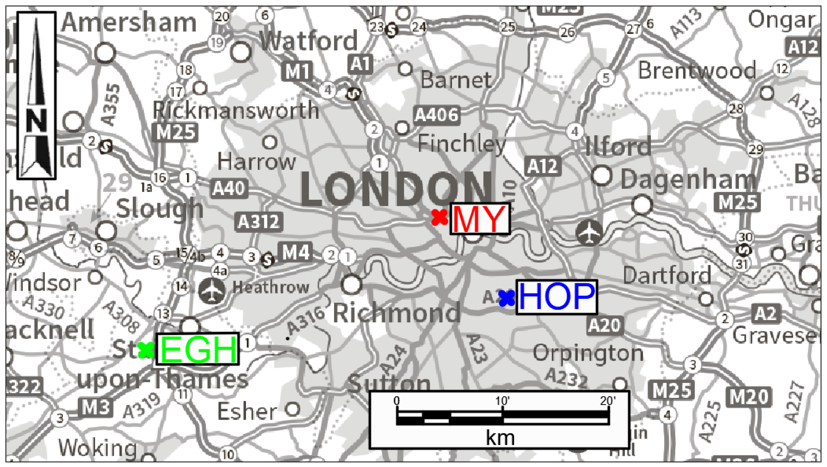
2.1. Measurement Locations

The locations of the measurement sites are shown in Figure 1.

The Marylebone Road (MY) urban traffic monitoring station located adjacent to the A501 Marylebone Road (51°31′21″ N, 0°09′17″ W) has been used for a large number of air quality research studies [5,33,55,65]. Sampling inlets are 3 m above ground and approximately 2 m from the edge of the carriageway. The road is a heavily congested east–west arterial route through Central London, with a high proportion of heavy-duty vehicles (HDVs), many of which are double decker buses. The station is located directly north of the boundary of the Ultra-Low Emission Zone (ULEZ). The surrounding tall buildings reduce the natural ventilation and generate a local “street-canyon”. Stationary queues of traffic are common, although the effect of this was reduced during the COVID-19 lockdown.

The Honor Oak Park (HOP) urban background monitoring station (51°26′59″ N, 0°02′15″ W) is located approximately 12 km southeast of MY. It is situated within a university sports ground and is approximately 100 m from the nearest road.

To improve the temporal coverage, further background CO₂ measurements were obtained from the Department of Earth Science at Royal Holloway University, Egham (EGH) (51°25′34″ N, 0°33′42″ W); this is located approximately 30 km southwest of MY [66]. EGH CO₂ background concentrations showed a reasonable correlation with HOP CO₂ background concentrations during the 12-month campaign (R² = 0.75). As such, the mean of these two sites was used to represent background CO₂ concentrations to improve temporal coverage for the dilution approach.

2.2. Atmospheric Measurements

MY and HOP measured a comprehensive array of particulate and gaseous pollutants. The 12-month campaign ran from 1 September 2019 until 31 August 2020.

2.2.1. PM₁₀ and PM_2.5 Mass

PM₁₀ and PM_2.5 mass concentrations were measured at MY and HOP using the Fidas 200 E (Palas, Germany); this uses Lorenz–Mie scattered light analysis of single particles to determine both PM mass and number concentrations [67]. These instruments were operated as part of the UK Automatic and Urban Rural Network (AURN); as such, they were subject to stringent quality assurance procedures [68]. The average uncertainty of the Fidas 200 E has previously been calculated as 7% for PM₁₀ and 10% for PM_2.5 at urban background and traffic locations and evaluated in accordance with BS EN 15267:2009 and the UK′s Monitoring Certification Scheme (MCERTS) Performance Standards for Continuous Ambient Air Quality Monitoring Systems, version 9.1 [67]. The benefits of using an optical scattering approach are that a single analyser can monitor the mass distribution of particles of a range of sizes at high time resolution. However, measurements which utilise optical techniques require assumptions to convert the particle counts into mass measurements, which can vary depending on the measurement location.

2.2.2. Elemental Composition

The elemental composition in PM₁₀ was measured at an hourly resolution using X-ray fluorescence (XRF). Two similar systems were used: Xact Model 625 at MY and Xact Model 625i at HOP, both from Cooper Environmental Services, USA. The instruments simultaneously measure up to 24 elements using reel-to-reel filter tape sampling [69,70]. The resulting PM deposit undergoes nondestructive XRF analysis to determine the metal content [71]. Both systems perform regular internal quality assurance checks; they are also manually checked against certified external standards and sample flows calibrated on a quarterly basis. Throughout the campaign, a < 5% deviation was observed between the measured concentration and standard mass for each element at both sites. Hourly sampling minimum detection limits (MDL) for the assessed elements are presented in Table S1. An uncertainty of 5–10% was previously calculated. This uncertainty is likely to be higher for concentrations close to the MDL, elements with potential for line interferences in multi-element samples, and for the lightest elements [72]. The systems previously showed good agreement with other high time resolution measurements (ion chromatography, aerosol mass spectrometry), and established filter-based laboratory analysis using inductively coupled plasma mass spectrometry (ICP-MS) [71,72]. During previous field deployments, the Xact′s XRF technique agreed well with the ICP-MS measurements of daily filter samples in all cases with a median R² of 0.93 and a median slope of 1.07 for the assessed elements [71]. During the 12-month campaign, the Xact′s data capture at MY was 75% and HOP was 70%.

2.2.3. Carbon Dioxide and Nitrogen Oxides

At MY, CO₂ concentrations were measured using a nondispersive infrared analyser (Model LI-820, LI-COR Inc, USA), which is a single closed path, dual wavelength detection system [73]. It measures CO₂ volume mixing ratios using an optical path thermostatically controlled infrared radiation detection system. The LI-820 was previously co-located with a PICARRO G2301 CRDS analyser (World Meteorological Organization′s (WMO) reference instrument) at the Greenhouse Gas Laboratory within the Department of Earth Sciences at Royal Holloway, University of London, and has an uncertainty of ±0.9 ppm (p < 0.05). At HOP, CO₂ concentrations were measured using cavity enhanced laser absorption (Multi-gas Carbon Emissions Gas Analyzer, Los Gatos Research, USA), which has an uncertainty of ±0.2 ppm (p < 0.05). The instrument uses Off-Axis Integrated Cavity Output Spectroscopy (OA-ICOS) technology, which allows the instrument to correct for water vapour dilution and absorption line broadening effects. During the campaign, both the LI-820 and the LGR Multi-gas Carbon Emissions Gas Analyzer were subject to regular on-site calibrations with a National Oceanic and Atmospheric Administration (NOAA) calibration gas at 800 ppm and a CO₂ free gas.

At EGH, CO₂ concentrations were measured using a cavity ring down spectrometer (Model Picarro G1301, Picarro, USA). The instrument has an uncertainty of ±0.05 ppm (p < 0.05) and is calibrated to the WMO X2007 CO₂ scale. The laboratory participates in WMO round robins and data are subject to robust quality assurance procedures as recommended by WMO/Global Atmospheric Watch (GAW).

Nitrogen oxides (NO_x) were measured at MY and HOP using chemiluminescence measurement techniques as part of the UK AURN, subject to stringent quality assurance procedures, and with an uncertainty < 15%.

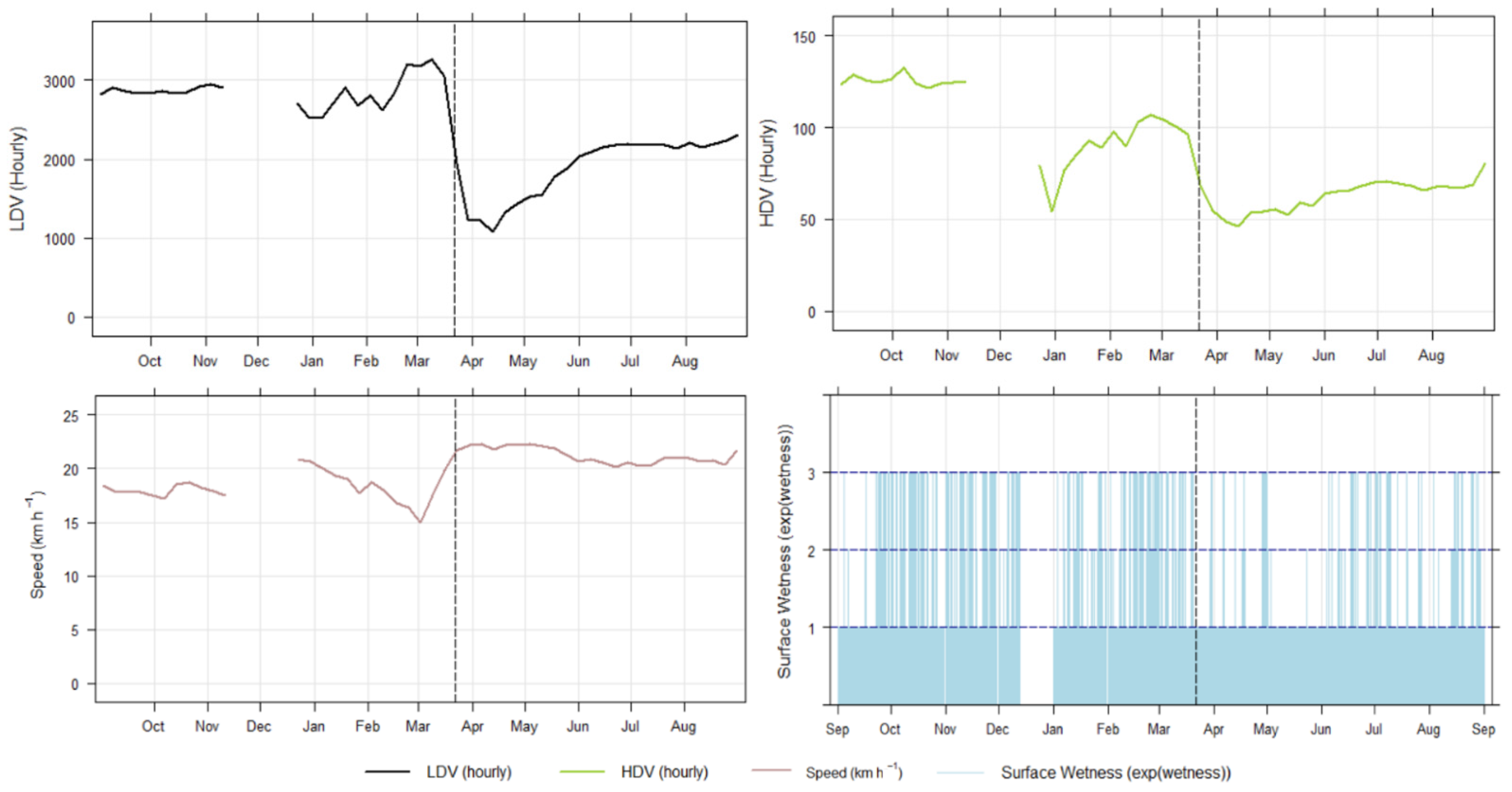
2.2.4. Traffic and Meteorological Data

An induction loop system (Marksman 660, Golden River, UK) was used to measure the number of light-duty vehicles (LDV) and heavy-duty vehicles (HDV) and instantaneous vehicle speed from all six lanes of Marylebone Road directly outside the measurement station. The instantaneous speed refers to the hourly average of the recorded vehicle speeds.

Background meteorological data were obtained from the WMO weather station (no. 03772) at Heathrow Airport (51°28′58.8′′ N, 0°27′0′′ W). The site is situated approximately 21 km west of Marylebone Road. This location provides synoptic meteorological conditions as is not disturbed by urban canopy layer interference, such as from buildings. Road surface wetness was measured using a sensor embedded in the Marylebone Road (Model DRS511, Vaisala, Finland) close to the monitoring station. The surface conditions were recorded as “dry (1)” (no humidity over the sensor), “moist (2)” (0.01–0.2 mm water film thickness over the sensor) and “wet (3)” (>0.2 mm) water film thickness over the sensor [74]. For the purpose of the non-exhaust emission factors, a wet road surface was considered any hourly period > 0.01 mm.

2.3. Calculating Non-Exhaust Concentrations

The results of a previous study at Marylebone Road identifying the elemental tracers for non-exhaust concentrations were used to estimate the contribution of non-exhaust emissions, shown in

Table 1. Particulate matter (PM) non-exhaust emission trace elements scaling factors [5].

Source	Trace Element	Scaling Factor
Brake Wear	Ba	91
Tyre Wear	Zn	50
Resuspension	Si	3.6

[5]. Concentrations for Ba, Zn, and Si were used to calculate the concentrations of brake wear, tyre wear, and resuspension, respectively, by multiplying the scaling factor and the elemental concentration. Ba is typically used as a filler in brake pads by most manufacturers. A scaling factor of 91 was applied to the roadside increment in Ba concentrations to determine brake wear concentrations as brake dust was found to comprise 1.1% Ba [5,28,75]. A scaling factor of 50 was applied to the roadside increment in Zn concentrations to determine tyre wear, based on 50% of the measured Zn arising from tyre wear and Zn comprising 1% (mass) of the tyre [5,39]. A scaling factor of 3.6 was applied to the roadside increment in Si concentrations to calculate the resuspension based on the earth′s crustal composition [5].

2.4. CO₂ Dilution Approach

A CO₂ dilution approach was used to generate non-exhaust emission factors for the existing vehicle fleets. CO₂ concentrations were measured at roadside and background (EGH/HOP) monitoring locations. The CO₂ dilution approach involved three main steps:

• A roadside CO₂ increment was obtained by subtracting the background from the roadside CO₂ concentrations:

  $$\Delta C{O}_2=C{O}_{2 Roadside}-C{O}_{2 Background}$$

  (1)

  where ΔCO₂ is the CO₂ roadside increment, CO_{2 Roadside} is the CO₂ concentrations at MY, and CO_{2 Background} is the mean of HOP and EGH concentrations. Only hours where there was a CO₂ increment greater than 3 ppm were used for the purpose of this assessment.
• A dilution factor for CO₂ was calculated by combining the speed-dependent tailpipe CO₂ emission factors based on the number of LDVs and HDVs recorded on each lane with ambient CO₂ increment measurements. This is represented in the following equation:

  $$dC{O}_2=\frac{E{F}_{CO2 LDV}\times n_{LDV}+E{F}_{CO2 HDV}\times n_{HDV}}{\Delta C{O}_2}$$

  (2)

  where dCO₂ is the hourly dilution estimation for CO₂, n_veh is the number of vehicles, and EF_{CO2; veh} is the CO₂ fleet emission factors (g/km) for light-duty (e.g., cars and vans) and heavy-duty (e.g., trucks and buses) vehicles, and ΔCO₂ is the CO₂ increment calculated in Equation (1). The CO₂ emission factors were obtained from the Department for Environment, Food, and Rural Affairs′ (Defra) Emission Factor Toolkit (V10.1) [76,77].
• The PM emission factors for Ba, Zn, and Si for the average of the fleet was calculated using the measured PM chemical composition data:

  $$E{F}_{x,Fleet}=\frac{\Delta C_x\times d}{n_{tot}}$$

  (3)

  where EF_x,Fleet is the total fleet average tracer emission factor (e.g., Ba/Zn/Si), ∆C_x is the measured mass concentration of the roadside increment for tracer “x”, d is the CO₂ dilution factor calculated in Equation (2), and n_tot is the total number of vehicles in the assessment period (e.g., one hour), where n_tot = n_LDV + n_HDV. This calculation provided an aggregated fleet emission factor, encompassing the entire 12-month campaign (where there was an appropriate roadside increment), covering variability in traffic volumes, speeds, and road surface wetness conditions.

3. Results

3.1. Atmospheric Measurement Campaigns

A summary of the PM₁₀, PM_2.5, key elemental concentrations at both sites, and the associated mean roadside increments are presented in

Table 2. Campaign average roadside (MY), background (HOP), and roadside increment (MY-HOP) concentrations (μg/m³/ng/m³).

	Marylebone Road	Honor Oak Park	Roadside Increment (MY-HOP)
	Mean	Mean	Mean	Roadside/Background Ratio
	μg/m3	μg/m3	μg/m3
PM10	17.14	13.20	3.94	1.3
PM2.5	9.82	8.29	1.53	1.2
	ng/m3	ng/m3	ng/m3
Ba	24	3	21	8.0
Cu	23	3	20	7.7
Fe	1695	259	1436	6.5
Zn	29	14	15	2.1
Si	354	287	67	1.2
Ca	372	253	119	1.5

. The roadside increments for PM₁₀ (3.94 μg/m³) and PM_2.5 (1.53 μg/m³) demonstrate that roadside concentrations were 1.2 to 1.3 times higher than background concentrations, and that traffic emissions contributed to both the coarse and fine fractions of PM. Background mean concentrations of Fe (259 ng/m³), Si (287 ng/m³), and Ca (253 ng/m³) were substantially higher than the other elements due to their abundance in crustal and soil material. Tracers associated primarily with brake wear had similar roadside over background ratios (e.g., Ba (8.0), Cu (7.7), Fe (6.5)), signifying that they shared similar source profiles at MY. The roadside/background ratio for tyre wear and resuspension tracers (Zn (2.1), Si (1.2) and Ca (1.5)) were lower than those associated with brake wear, suggesting sources with lower roadside emission strengths. The roadside incremental results were in broad agreement with previous studies which showed that these elements were typical of road traffic sources [5,21,25].

Figure 2 shows the weekly roadside, background and increment concentrations of PM₁₀, PM_2.5, CO₂, Ba, Zn, and Si. Figure S1 shows the daily average variations in CO₂ concentrations. The start of lockdown coincided with a pollution episode from western Europe, resulting in elevated mixing ratios at HOP and thus only a negligible increment in PM₁₀ and PM_2.5. Nevertheless, it is clear that the CO₂, PM_2.5 and (to a lesser extent) PM₁₀ roadside increments reduced at the start of the UK lockdown on 23 March 2020. The impact on the non-exhaust emission tracers (Ba, Zn, and Si) is not so clear. It should be noted that instrument failure occurred for the elemental composition measurements at MY from the beginning of lockdown, and at HOP prior to the start of lockdown. These notable PM composition data set gaps have implications for direct comparison between the PM mass traffic increments and the elemental composition data.

Figure 3 shows a number of important factors which affect these tracer emissions, including average hourly LDV and HDV volume, vehicle speed, and road surface wetness during the campaign. Prior to lockdown, the average hourly traffic volume on the six lanes at Marylebone Road was 2872 (3.6% HDV), whereas during lockdown, there was an average of 1944 (3.2% HDV) vehicles. This equates to a reduction of 31% in LDVs and 40% in HDVs. The changes in traffic volume caused by lockdown meant that the average measured instantaneous speed was 18 km h⁻¹ before lockdown, and 21 km h⁻¹ during lockdown, which equates to a 15% increase. Overall congestion also reduced during lockdown as the minimum average hourly speed increased from 8 km h⁻¹ to 12 km h⁻¹. The weekly average road surface conditions are displayed in a logarithmic scale, where higher average road surface wetness conditions are reflected by higher logarithmic units. Before lockdown (autumn and winter), 44% of the hourly road surface data had periods with moist/wet road surface conditions, whereas during lockdown (spring and summer periods), moist/wet road surface conditions only accounted for 9% of the hourly road surface data.

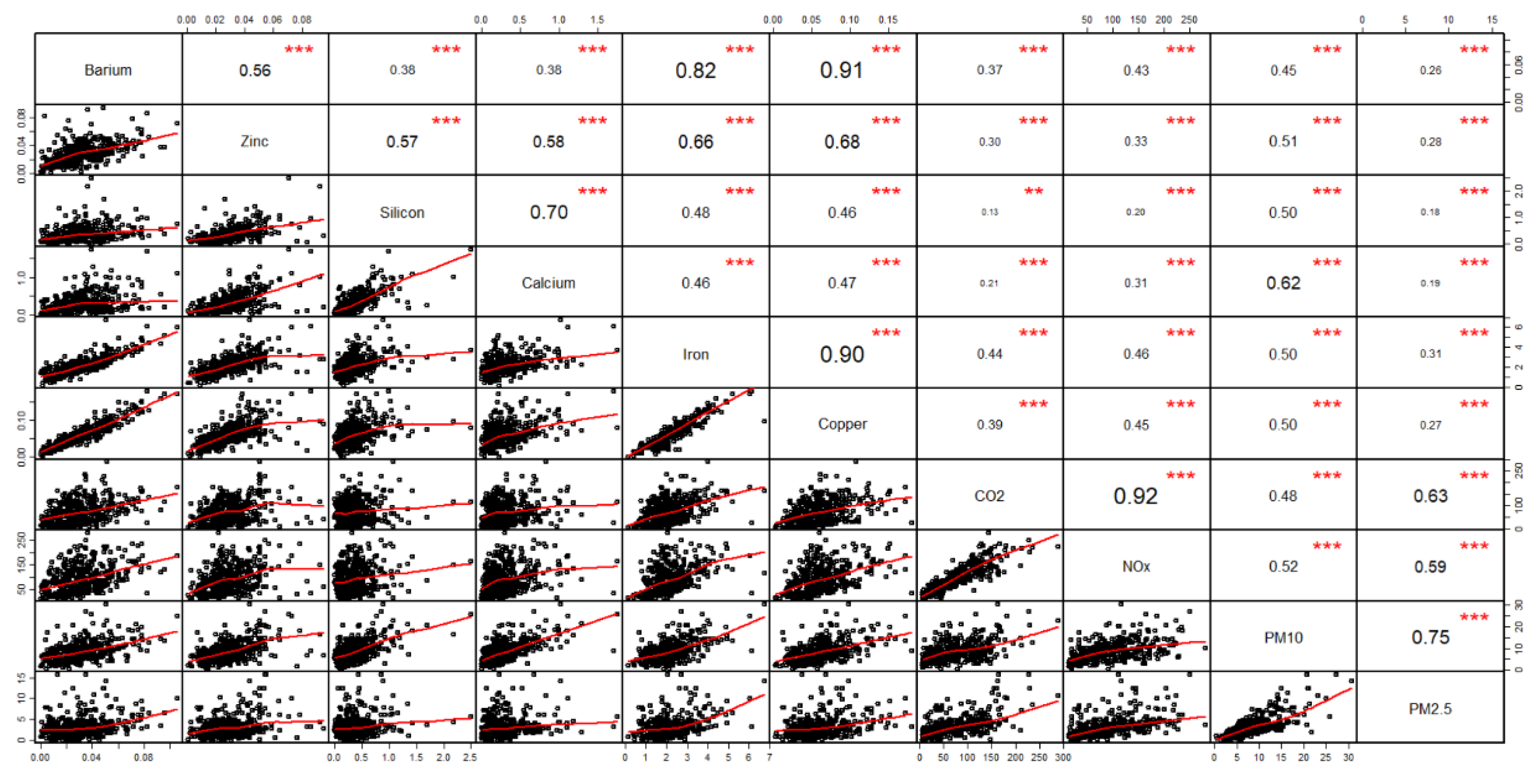
3.1.1. Measurement Correlations

Spearman correlation coefficients of the Marylebone Road increments for PM₁₀ and PM_2.5, key trace elements (Ba, Zn, Si, Ca, Fe, Cu), and exhaust gases (NO_x/CO₂) are displayed in Figure 4. The correlation coefficient values and p-value symbols are shown on the top of diagonal and bivariate scatter plots with a monotonic smoothing curve are displayed on the bottom diagonal. Correlations generally show a p-value ≤ 0.001 (***) due to the long sampling period and high time resolution of the measurements.

Figure 4 shows that strong correlations exist between the increments of PM (PM₁₀ and PM_2.5 = 0.75) and the increments of exhaust gases (NO_x and CO₂ = 0.92). The increments of PM also share moderate relationships with NO_x (PM₁₀ = 0.52/PM_2.5 = 0.59) and CO₂ (PM₁₀ = 0.48/PM_2.5 = 0.63). Whilst the causes of these emissions are dissimilar, the correlations indicate that they share similar driving processes and influences of atmospheric dispersion.

Ba was used to represent brake wear emissions in this study and had strong correlations with the traffic increments of Fe (0.82) and Cu (0.94). Fe is the most abundant material in brake discs and Cu is an important brake friction material which improves the thermal conductivity and decreases the wear rate of brake pads. Zn, which represents tyre wear, is relatively common in both anthropogenic and natural sources. However, the Zn traffic increment correlated moderately well with the traffic increments of Ba (0.56), Fe (0.66), and Cu (0.68), suggesting that the tyre wear and brake wear tracers incorporated similar profiles and dispersion influences. In addition to being used as brake material, Fe and Cu are also used in small quantities to make up the composition in tyres (e.g., steel cords and alloys) and are a component of exhaust PM emissions (e.g., fuel additives, engine wear), whilst Zn is used in brake pads. Si, which represents a tracer for resuspension, had a strong correlation with Ca (0.70). These two elements, which are primarily found in the earth′s crustal material, shared moderate relationships with PM₁₀ (Si = 0.50/Ca = 0.62).

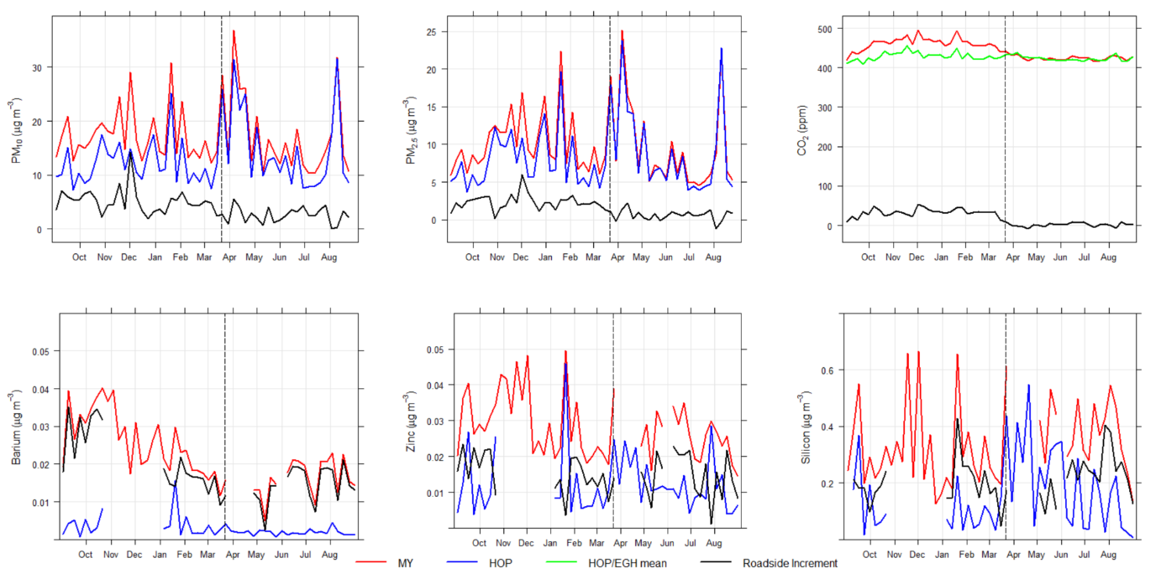
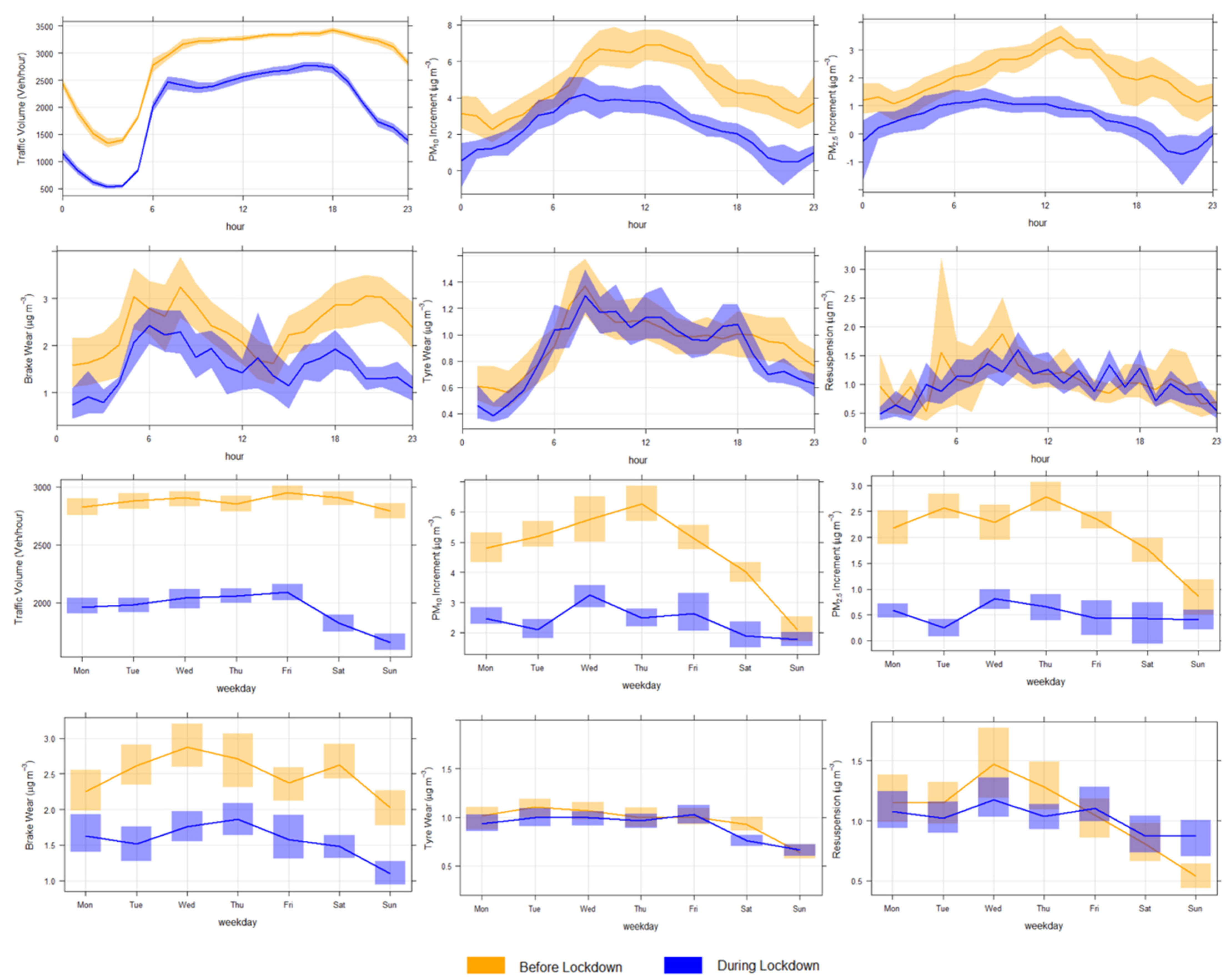
3.1.2. PM₁₀, PM_2.5, and Non-Exhaust Traffic Concentrations

Non-exhaust concentrations were calculated using the non-exhaust scaling factors described above. The mean PM₁₀ and PM_2.5 traffic increments and the brake wear, tyre wear, and resuspension concentrations before and during lockdown are shown in

Table 3. Average PM₁₀ and PM_2.5 traffic increment and non-exhaust emission concentrations at Marylebone Road during the campaign (μg/m³).

Source	Overall	Pre-Lockdown	Lockdown	Change
	μg/m3	μg/m3	μg/m3	μg/m3
PM10 Increment	3.9	4.7	2.4	−2.3
PM2.5 Increment	1.5	2.1	0.5	−1.6
Brake Wear	1.9	2.6	1.6	−1.0
Tyre Wear	1.0	1.0	1.0	0.0
Resuspension	1.1	1.1	1.1	0.0

, whilst the diurnal patterns and day of the week variations are shown in Figure 5. The PM₁₀ and PM_2.5 traffic increments showed substantial decreases in concentrations as a result of lockdown, reducing by 49% and 76%, respectively. Figure 5 shows that the greatest reductions in these concentrations were seen during periods with higher traffic volumes (e.g., daytime and weekdays). In line with previous studies at MY [5,10], brake wear was the highest emission source, contributing 1.9 μg/m³ during this annual campaign. However, there was a 39% reduction in brake wear concentrations during lockdown, reducing from 2.6 μg/m³ before lockdown to 1.6 μg/m³ during lockdown. Average tyre wear concentrations remained stable both before and during lockdown and contributed 1 μg/m³. Resuspension concentrations contributed to 1.1 μg/m³ at MY and also did not show a clear difference in emissions before and during lockdown. The non-exhaust concentrations generally illustrated diurnal patterns which are typical of traffic sources, with concentration peaks during morning rush hour, although subsequent increases during evening rush hour were not that clear for tyre wear and resuspension. Small reductions in non-exhaust concentrations were also seen during the weekend. Direct comparisons between the PM mass and non-exhaust emissions should be avoided due to dataset gaps at HOP (prior to lockdown) and MY (at the start of lockdown).

3.2. Emission Factors

PM₁₀, brake wear, tyre wear, and resuspension emission factors were developed using the CO₂ dilution described in Section 2.4.

3.2.1. CO₂ Dilution Approach

The CO₂ dilution approach assumed that the background monitoring stations were not affected by local emission sources. Figure S2 illustrates the background CO₂ mixing ratios at HOP and MY based on wind speed and wind direction. The highest mixing ratios occurred during periods with very low wind speeds, typically during temperature inversions when there was a lack of dispersion. EGH also showed slightly elevated mixing ratios during easterly wind directions, which is perhaps characterised by local emission sources from the M25 motorway and Heathrow Airport at low wind speeds and additional London emission sources at higher wind speeds. The HOP polar plots did not suggest any specific directionality from local emission sources. The CO₂ dilution approach was only applied to hours where there was considered a suitable CO₂ traffic increment at MY. The CO₂ traffic increments at MY before lockdown and during lockdown are presented by time of day and day of week in Figure S3. There was a substantial reduction in CO₂ mixing ratios as a result of lockdown. The recorded traffic conditions and the use of associated CO₂ emission factors encompassed these two periods and enabled the generation of the CO₂ dilution factors, which varied during the campaign and were dependent on seasonality and time of the day. Higher dilution factors were found in summer (average: 2.5 × 10⁷ to 3.5 × 10⁷), mid dilution factors in spring/autumn (average: (1.7 × 10⁷ to 2.5 × 10⁷), and lower dilution factors in winter (average: 1.2 × 10⁷ to 1.7 × 10⁷). The dilution factors also varied by time of the day, with lower dilution factors from 00:00 to 06:00, mid dilution factors from 06:00 to 18:00, and higher dilution factors from 18:00 to 00:00. Whilst this campaign incorporated a 12-month period, the systematic temporal variability in the dilution factor was an important consideration, particularly if undertaking the CO₂ dilution approach for short-term campaigns.

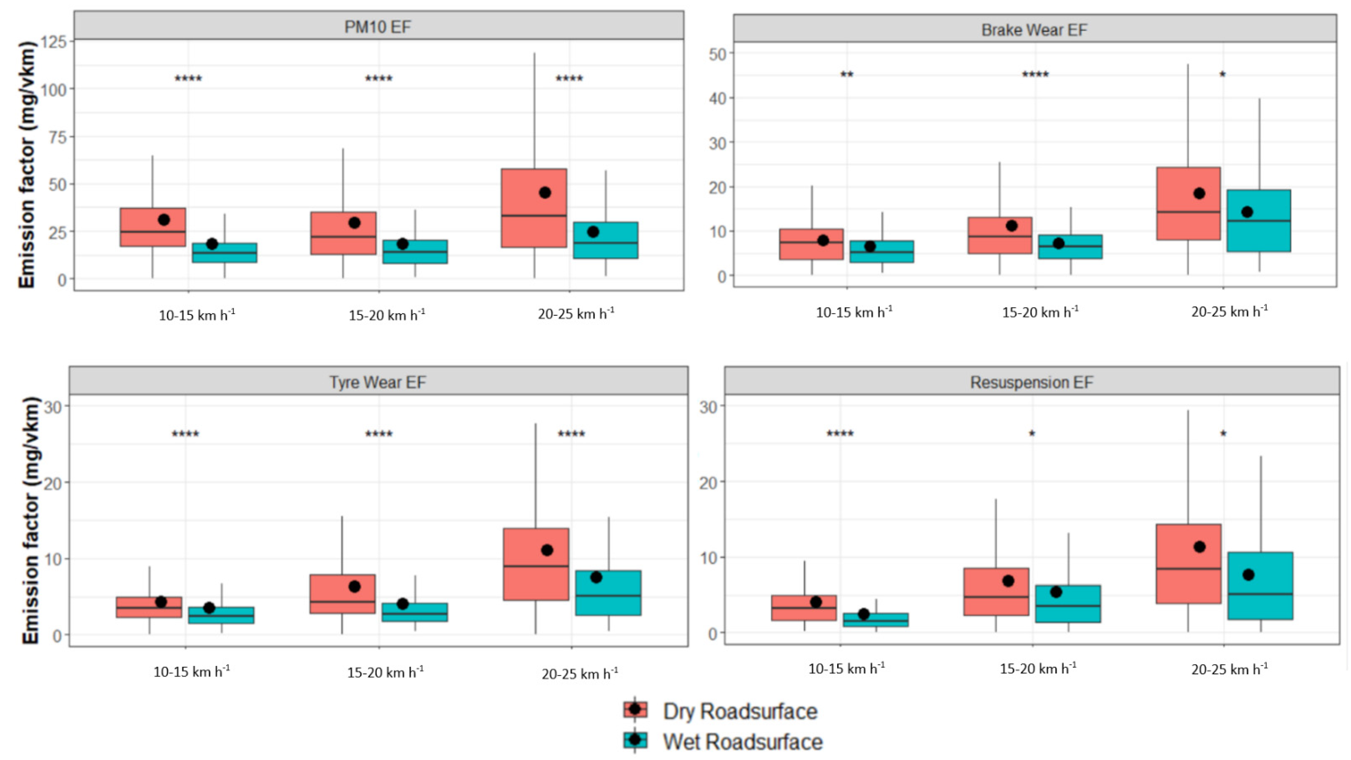
3.2.2. Non-Exhaust Emission Factors

The CO₂ dilution approach was applied to the non-exhaust concentrations to obtain emission factors. A summary of the fleet-average emission factors by measured speed and road surface wetness conditions is presented in

Table 4. Average fleet non-exhaust emission factors at Marylebone Road by speed and surface wetness (mg vkm⁻¹).

Emission Factor (mg vkm−1)	Dry Road Surface			Wet Road Surface			Combined
	10–15 kmh−1	15–20 kmh−1	20–25 kmh−1	10–15 kmh−1	15–20 kmh−1	20–25 kmh−1	10–25 kmh−1
PM10	30.8	29.0	45.4	18.2	18.1	24.5	34.5
Brake Wear	7.9	11.1	18.4	6.5	7.1	14.1	12.9
Tyre Wear	4.2	6.3	11.0	3.5	4.0	7.5	7.8
Resuspension	4.0	6.8	11.3	2.4	5.3	7.5	8.0

and Figure 6. Changes in speed and road surface wetness conditions were tested using the Wilcoxon signed-rank and Kruskal–Wallis tests.

Average fleet emission factors for the combined road surface conditions were 34.5 mg vkm⁻¹ for PM₁₀, 12.9 mg vkm⁻¹ for brake wear, 7.8 mg vkm⁻¹ for tyre wear, and 8.0 mg vkm⁻¹ for resuspension. Lower non-exhaust emission factors were seen during slow speeds and wet road surface conditions; higher emission factors were seen during dry conditions and faster speeds. The emission factors showed differences based on overall changes in speed bin during both dry and wet conditions—and between all individual speed bins in dry conditions. However, changes in speed were not considered as significant for PM₁₀ in both dry and wet road surface conditions between 10 and 15 km h⁻¹ and 15 and 20 km h⁻¹, for brake wear in wet conditions between 10 and 15 km h⁻¹ and 15 and 20 km h⁻¹, and for resuspension in wet conditions between 15 and 20 km h⁻¹ and 20 and 25 km h⁻¹. Figure 6 demonstrates the changes in road surface wetness conditions in the emission factors, although the p-value varied depending on the emission source and speed bin. All non-exhaust emission sources showed changes in emission factors based on road surface wetness condition, although tyre wear showed the most notable changes.

The sum of the combined non-exhaust emission factors (28.7 mg vkm⁻¹) represented 83% of the total PM₁₀ emission factors (34.5 mg vkm⁻¹). This indicates that during the measurement campaign, the exhaust PM₁₀ emission factor for the average fleet was 5.8 mg vkm⁻¹, which was 17% of total vehicle PM₁₀ emissions. The non-exhaust emission factors increased with average vehicle speed during both wet and dry conditions. The overall PM₁₀ emission factors, which incorporated both exhaust and non-exhaust emissions, did not have a clear relationship with speed.

4. Discussion

4.1. Brake Wear

Brake wear emissions, which contributed on average to 1.9 μg/m³, were highly dependent upon the braking frequency and conditions under which braking events occurred. The incidence of braking and the high traffic volumes and congested conditions at Marylebone Road led to stop–start traffic movements and frequent braking, causing brake wear to be the highest PM emission source at this location. This contribution is expected to be reduced at roads where there is less frequent braking, such as rural roads and motorways. The diurnal and day of the week patterns demonstrate that brake wear concentrations were sensitive to changes in traffic volume and congestion. Brake wear significantly decreased during lockdown, with 32% less traffic volume leading to a similar reduction in concentrations. The emission factors established that brake wear emissions were sensitive to changes in vehicle speed and road surface wetness conditions. Increases in measured speed was associated with higher acceleration and deceleration rates, whilst more aggressive braking would lead to higher brake temperatures, and therefore brake wear emissions [16,17,25].

The average fleet brake wear emission factor (12.9 mg vkm⁻¹) developed in this study was compared with the EMEP/EEA Guidebook′s urban emission factors produced for LDVs (motorcycle/private cars/LGV average = 11.9 mg vkm⁻¹) and HDVs (rigid/artic HGV′s/bus average = 51.9 mg vkm⁻¹) [6,26,78]. Using the Guidebook′s LDV/HDV emission factor split and the campaign′s average fleet composition, it was calculated that brake wear emission factors for LDVs were 11.5 mg vkm⁻¹ and HDVs were 50.3 mg vkm⁻¹. This campaign′s emission factors show excellent agreement with the estimates used for the reporting of the UK NAEI and are suitable to use in other urban environments with similar fleet compositions to London. A higher number of vehicle axles and increased vehicle weight explain the over 4-fold increase in HDV emission factors. However, it is not yet clear whether the heavier weight of battery electric vehicles would increase the frictional component of brake wear, although regenerative braking is likely to offset any increase in brake wear¹⁰. Further work is needed to expand the range of assessed vehicle speeds and to determine the impact of ambient atmospheric temperature and humidity on brake wear emission factors. Moreover, there remains uncertainty associated with the Ba scaling factors used to determine brake wear concentrations. In particular, whilst the scaling factors assume that the traffic increment is only a tracer for brake wear, Ba is also found at trace concentrations in oil lubricants and the earth′s crustal material and so would therefore also be seen in the PM exhaust component and crustal resuspension material, albeit to a relatively small extent.

The influence of lockdown has shown that urban brake wear mitigation strategies would benefit primarily from traffic volume reductions. However, the introduction of technology such as regenerative braking and low emission disc brake systems (which have greater frictional wear resistance) could also play an important role in reducing brake wear emissions in the future.

4.2. Tyre Wear

Tyre wear was less prevalent than brake wear, contributing on average to 1 μg/m³. Despite moderate correlations between Zn and Ba during the campaign, differences in the roadside/background ratios, concentrations, and the developed emission factors illustrate that there were also important differences between brake wear and tyre wear emission characteristics. Interestingly, tyre wear did not decrease in a similar manner to brake wear as a result of lockdown. However, the diurnal and day of week patterns demonstrate that changes in traffic volumes affected tyre wear concentrations when speed and road surface wetness conditions remained stable (e.g., during weekend and nighttime). Speed has previously been shown to affect tyre wear emissions due to increases in tyre temperature and mechanical wear, whilst wet road surface conditions can act as a lubricant between the road and the tyre and can reduce the extent of tyre/road friction—and therefore emissions [64]. Tyre wear emission factors exhibited important changes due to higher vehicle speeds at both dry and wet road surfaces. Higher average vehicle speeds and lower road surface wetness conditions seen during lockdown were therefore predicted to have offset the lower traffic volumes which occurred during this period. In addition to vehicle and road surface conditions, laboratory studies indicate that specific tyre characteristics (e.g., size, tread depth, pressure and temperature, chemical composition, accumulated mileage, age, and quality) are also important in determining tyre wear emissions [72]. Lockdown may have resulted in tyres with higher accumulated mileage (due to the closure of garages), although it is uncertain whether this would affect tyre wear emissions.

The fleet average PM₁₀ emission factors (7.8 mg vkm⁻¹) were compared with the EMEP/EEA Guidebook′s urban emission factors for LDVs (8.7 mg vkm⁻¹) and HDVs (29.7 mg vkm⁻¹) [6,26,78]. Using the same approach as brake wear, it was determined that tyre wear emission factors for LDVs were 7.0 mg vkm⁻¹ and HDVs were 29.6 mg vkm⁻¹ [78]. This shows very good agreement with the emission factors used in the reporting of UK NAEI. A higher number of vehicle axles and increased vehicle weight played important roles in the 4-fold increase in HDV tyre wear emission factor (similarly to brake wear). Thus, further consideration is needed with respect of emission factors from heavier battery electric vehicles, which may result in more tyre wear emissions than the current vehicle fleet. Overall, the tyre wear emission factors are also considered suitable for urban environments with similar vehicle fleet compositions, as Zn is used consistently in tyres to vulcanize rubber. However, further work is needed to better understand the relationship between a greater range of vehicle speeds, whilst a key limitation of this research is that the tyre wear concentrations were based on Zn scaling factors, an element which only represents 1–2% of the tyre. Indeed, a wide range of chemical compounds are used to manufacture tyres.

Based on this research, urban tyre wear mitigation strategies should focus on reducing traffic volume and average vehicle speed, although the latter may have an adverse impact on exhaust emissions. Further measurements which incorporate organic rubbers and microplastics would provide important datasets for source apportionment studies.

4.3. Resuspension

Resuspension concentrations also demonstrated a nonlinear relationship with traffic volume. In particular, the changes in traffic volume during lockdown stipulated that increasing the number of vehicles did not correspond to increases in resuspension concentrations, whilst there was a negative correlation between resuspension tracer elements and exhaust gases. However, the diurnal and day of the week concentrations showed that resuspension did increase during rush hour periods and reduced on Sunday. As emission factors are intrinsically related to the number of vehicles, the PM road dust deposition rate was assumed to be proportional to the traffic flow rate [49]. However, it was established that a smaller number of vehicles generated comparable resuspension concentrations. This is because the available road dust for resuspension is removed from the road rapidly—further emissions are not proportionally increased by higher traffic volume²⁷. Whilst Marylebone Road is likely to continuously generate a road dust basin from traffic and other urban sources, the use of only silicon as a tracer for resuspension would not necessarily account for this. This may have resulted in an underestimation of resuspension concentrations and emissions as it has been suggested that up to 40% of road dust could be removed from a given part of a paved road after the passage of a single vehicle, although much of this material could be deposited back on the road surface [47,48]. On the other hand, the brake and tyre wear emission factors may have included a component of resuspended material. Separating resuspension from direct non-exhaust emissions is complex and requires further statistical analysis. Changes in vehicle speeds and road surface wetness conditions were established to have an important role in changing the resuspension emissions during dry road surface conditions, possibly as a result of increased vehicle-induced turbulence. However, the impact of speed was not as significant during wet conditions, as rainfall causes the aggregation of particles and their surface runoff [52,54]. Urban resuspension mitigation strategies would therefore benefit from reducing average vehicle speed, whilst regular street cleaning would also reduce the available material for resuspension. Whilst vehicle-based emission factors are needed for simplicity and practicality, the influence of other variables such as wind direction, wind speed, vehicle size/weight, and silt loading (which were not assessed) can affect the physical dynamics of resuspension, potentially also having an important role [57].

Nevertheless, the average vehicle fleet resuspension emission factors were comparable to previous studies. The emission factors (8.0 mg vkm⁻¹) were slightly lower than those previously estimated from a Marylebone Road campaign in 2009 which predicted (average fleet) 10 mg vkm⁻¹ using a NO_x dilution approach⁸. Exhaust emission reductions since this earlier campaign would have also reduced resuspension emissions as there is less exhaust PM deposited on the road, although this would not necessarily have been seen by using Si as a tracer. This study′s emission factors were much lower than emission factors generated in Barcelona (22.7 mg vkm⁻¹), a Mediterranean city with lower rainfall/moisture, vegetative cover, and higher road dust than in London [45]. On the other hand, the emission factors were comparable with emission factors calculated in 2016 for inner-city roads in Paris during an urban campaign, a city with a similar climate to London, which predicted average fleet emission factors of 5.4–9 mg vkm⁻¹ using a silt-loading methodology [10,49,52]. Taking into account the limitations of vehicle-based resuspension emission factors, these emission factors are considered appropriate for use in busy traffic environments with similar meteorological conditions to London.

5. Summary and Conclusions

A 12-month measurement campaign was undertaken at Marylebone Road and Honor Oak Park to quantify non-exhaust emissions using highly time-resolved PM₁₀ and elemental composition measurements. To determine the non-exhaust emission concentrations, previously developed scaling factors were applied to the measured concentrations of Ba (brake wear), Zn (tyre wear), and Si (resuspension), respectively. A CO₂ dilution approach was undertaken to predict the fleet average non-exhaust emission factors, an approach which had previously been used with NO_x as the dilution gas. There were systematic temporal variabilities in the CO₂ dilution factor, which is an important consideration, particularly if undertaking the CO₂ dilution approach for short-term campaigns.

The roadside increment (MY–HOP) for the PM₁₀ and PM_2.5 mass and non-exhaust sources varied substantially over the course of the campaign. A comparison between the results of pre-lockdown and lockdown concentrations showed that the overall PM₁₀ and PM_2.5 traffic increments reduced by 49% and 76%, respectively. The predicted non-exhaust concentrations showed that brake wear was the leading non-exhaust emission source at MY. However, despite a reduction in traffic volumes of 32%, there was only a noticeable decrease in brake wear concentrations out of the non-exhaust emission sources. Tyre wear and resuspension concentrations did not show a discernable difference caused by lockdown, signifying complex relationships with traffic volume.

The non-exhaust emission factors were dependent upon speed and road surface wetness. During lockdown, reductions in road surface wetness conditions and increases in vehicle speed offset the reductions in traffic volumes and explained, in part, why tyre wear and resuspension did not reduce during lockdown. The brake and tyre wear emission factors showed very good agreement with the EMEP/EEA Guidebook′s emission factors, whilst the resuspension emission factors were also comparable to previous studies. Despite this, there remains uncertainty associated with the non-exhaust scaling factors, vehicle splits, and the applicability of the emission factors on a wider scale. Moreover, this research emphasises the importance of also considering meteorological conditions in addition to traffic volume and speed. Indeed, vehicle-based emission factors are needed for simplicity and practicality; however, the influence of other variables such as wind direction, wind speed, vehicle size/weight and silt loading can affect the physical dynamics of non-exhaust emissions. Further measurements, which incorporate a wider variability in vehicle speeds and chemical tracers, should be undertaken to better understand these processes and to improve their representativeness, whilst advanced source apportionment of the PM measurement data will enable improved understanding of their contribution.

References

1. Committee on the Medical Effects of Air Pollutants (COMEAP). The Effects of Long-Term Exposure to Ambient Air Pollution on Cardiovascular Morbidity: Mechanistic Evidence; Committee on the Medical Effects of Air Pollutants: Chilton, UK, 2018. [Google Scholar]
2. World Health Organization (WHO). Ambient Air Pollution: A Global Assessment of Exposure and Burden of Disease; World Health Organization: Geneva, Switzerland, 2016. [Google Scholar]
3. Font, A.; Guiseppin, L.; Blangiardo, M.; Ghersi, V.; Fuller, G.W. A tale of two cities: Is air pollution improving in Paris and London? Environ. Pollut. 2019, 249, 1–12. [Google Scholar] [CrossRef] [PubMed]
4. Joshi, A.; Johnson, T. Gasoline particulate filters—A review. Emiss. Control Sci. Technol. 2018, 4, 219–239. [Google Scholar] [CrossRef]
5. Harrison, R.M.; Jones, A.M.; Gietl, J.; Yin, J.; Green, D.C. Estimation of the contributions of brake dust, tire wear, and resuspension to nonexhaust traffic particles derived from atmospheric measurements. Environ. Sci. Technol. 2012, 46, 6523–6529. [Google Scholar] [CrossRef] [PubMed]
6. Air Quality Expert Group (AQEG). Non-Exhaust Emissions from Road Traffic; Defra: London, UK, 2019. [Google Scholar]
7. Committee on the Medical Effects of Air Pollutants (COMEAP). Statement on the Evidence for Health Effects Associated with Exposure to Non-Exhaust Particulate Matter from Road Transport; Committee on the Medical Effects of Air Pollutants: Chilton, UK, 2020. [Google Scholar]
8. Eionet. Projected Emissions (March 2020 Submission). Updated 2020. Available online: http://cdr.eionet.europa.eu/gb/un/clrtap/projected/envxmo40w/overview (accessed on 12 October 2020).
9. Ntziachristos, L.; Boulter, P. EMEP/EEA Air Pollutant Emission Inventory Guidebook 2019; EMEP/EEA: Copenhagen, Denmark, 2019. [Google Scholar]
10. European Environment Agency. Directive (EU) 2016/2284 of the European Parliament and of the Council of 14 December 2016 on the reduction of national emissions of certain atmospheric pollutants, amending directive 2003/35/EC and repealing directive 2001/81/EC. Off. J. Eur. Union 2016, 344, 1–31. Available online: http://data.europa.eu/eli/dir/2016/2284/oj (accessed on 11 August 2020).
11. Committee on Climate Change. Net Zero: The UK’s Contribution to Stopping Global Warming. 2019. Available online: https://www.theccc.org.uk/publication/net-zero-the-uks-contribution-to-stopping-global-warming/ (accessed on 15 August 2020).
12. UN Economic Commission for Europe (UNECE). Convention on Long-Range Transboundary Air Pollution (LRTAP); European Environment Agency: Copenhagen, Denmark, 2020. [Google Scholar]
13. Timmers, V.R.J.H.; Achten, P.A.J. Non-exhaust PM emissions from electric vehicles. Atmos. Environ. 2016, 134, 10–17. [Google Scholar] [CrossRef]
14. Beddows, D.C.; Harrison, R.M. PM10 and PM2.5 emission factors for non-exhaust particles from road vehicles: Dependence upon vehicle mass and implications for battery electric vehicles. Atmos. Environ. 2021, 244, 117886. [Google Scholar] [CrossRef]
15. Hagino, H.; Oyama, M.; Sasaki, S. Laboratory testing of airborne brake wear particle emissions using a dynamometer system under urban city driving cycles. Atmos. Environ. 2016, 131, 269–278. [Google Scholar] [CrossRef] [Green Version]
16. Garg, B.D.; Cadle, S.H.; Mulawa, P.A.; Groblicki, P.J.; Laroo, C.; Parr, G.A. Brake wear particulate matter emissions. Environ. Sci. Technol. 2000, 34, 4463–4469. [Google Scholar] [CrossRef]
17. Sanders, P.G.; Xu, N.; Dalka, T.M.; Maricq, M.M. Airborne brake wear debris: Size distributions, composition, and a comparison of dynamometer and vehicle tests. Environ. Sci. Technol. 2003, 37, 4060–4069. [Google Scholar] [CrossRef]
18. Gustafsson, M.; Blomqvist, G.; Gudmundsson, A.; Dahl, A.; Jonsson, P.; Swietlicki, E. Factors influencing PM10 emissions from road pavement wear. Atmos. Environ. 2009, 43, 4699–4702. [Google Scholar] [CrossRef]
19. Park, I.; Kim, H.; Lee, S. Characteristics of tire wear particles generated in a laboratory simulation of tire/road contact conditions. J. Aerosol Sci. 2018, 124, 30–40. [Google Scholar] [CrossRef]
20. Mathissen, M.; Grigoratos, T.; Lähde, T.; Vogt, R. Brake wear particle emissions of a passenger car measured on a chassis dynamometer. Atmosphere 2019, 10, 556. [Google Scholar] [CrossRef] [Green Version]
21. Charron, A.; Polo-Rehn, L.; Besombes, J.-L.; Golly, B.; Buisson, C.; Chanut, H.; Marchand, N.; Guillaud, G.; Jaffrezo, J.-L. Identification and quantification of particulate tracers of exhaust and non-exhaust vehicle emissions. Atmos. Chem. Phys. Discuss. 2019, 19, 5187–5207. [Google Scholar] [CrossRef] [Green Version]
22. Dante, R.C. Handbook of Friction Materials and Their Applications; Woodhead Publishing Ltd.: Cambridge, UK, 2015; pp. 1–6. [Google Scholar]
23. Crilley, L.R.; Lucarelli, F.; Bloss, W.J.; Harrison, R.M.; Beddows, D.C.; Calzolai, G.; Nava, S.; Valli, G.; Bernardoni, V.; Vecchi, R. Source apportionment of fine and coarse particles at a roadside and urban background site in London during the 2012 summer ClearfLo campaign. Environ. Pollut. 2017, 220, 766–778. [Google Scholar] [CrossRef] [PubMed] [Green Version]
24. Visser, S.; Slowik, J.G.; Furger, M.; Zotter, P.; Bukowiecki, N.; Canonaco, F.; Flechsig, U.; Appel, K.; Green, D.C.; Tremper, A.H.; et al. Advanced source apportionment of size-resolved trace elements at multiple sites in London during winter. Atmos. Chem. Phys. Discuss. 2015, 15, 11291–11309. [Google Scholar] [CrossRef] [Green Version]
25. Grigoratos, T.; Martini, G. Brake wear particle emissions: A review. Environ. Sci. Pollut. Res. 2015, 22, 2491–2504. [Google Scholar] [CrossRef] [Green Version]
26. Grigoratos, T.; Martini, G. Non-Exhaust Traffic Related Emissions. Brake and Tyre Wear PM. 2014. Available online: https://publications.jrc.ec.europa.eu/repository/bitstream/JRC89231/jrc89231-online%20final%20version%202.pdf (accessed on 5 November 2020).
27. Amato, F.; Cassee, F.R.; Van Der Gon, H.A.D.; Gehrig, R.; Gustafsson, M.; Hafner, W.; Harrison, R.M.; Jozwicka, M.; Kelly, F.J.; Moreno, T.; et al. Urban air quality: The challenge of traffic non-exhaust emissions. J. Hazard. Mater. 2014, 275, 31–36. [Google Scholar] [CrossRef]
28. Thiyagarajan, V.; Kalaichelvan, K.; Vijay, R.; Singaravelu, D.L. Influence of thermal conductivity and thermal stability on the fade and recovery characteristics of non-asbestos semi-metallic disc brake pad. J. Braz. Soc. Mech. Sci. Eng. 2015, 38, 1207–1219. [Google Scholar] [CrossRef]
29. Jang, J. Brake friction materials. In Encyclopaedia of Tribology; Wang, Q.J., Chung, Y., Eds.; Springer: Boston, MA, USA, 2013. [Google Scholar]
30. Güney, B.; Öz, A. Microstructure and chemical analysis of vehicle brake wear particle emissions. Eur. J. Sci. Technol. 2020, 19, 633–642. [Google Scholar] [CrossRef]
31. Breuer, B.; Bill, K. Bremsenhandbuch, 5th ed.; Springer Vieweg: Wiesbaden, Germany, 2017. [Google Scholar]
32. Karthikeyan, S.S.; Balakrishnan, E.; Meganathan, S.; Balachander, M.; Ponshanmugakumar, A. Elemental analysis of brake pad using natural fibres. Mater. Today Proc. 2019, 16, 1067–1074. [Google Scholar] [CrossRef]
33. Harrison, R.M.; Beddows, D.C.S.; Dall’Osto, M. PMF Analysis of wide-range particle size spectra collected on a major highway. Environ. Sci. Technol. 2011, 45, 5522–5528. [Google Scholar] [CrossRef]
34. Grigoratos, T.; Gustafsson, M.; Eriksson, O.; Martini, G. Experimental investigation of tread wear and particle emission from tyres with different treadwear marking. Atmospheric Environment. 2018, 182, 200–212. Available online: http://www.sciencedirect.com/science/article/pii/S1352231018302036 (accessed on 29 January 2021). [CrossRef]
35. Kesarkar, A.P.; Biswal, A.; Kesarkar, A.P.; Mor, S.; Ravindra, K. High resolution vehicular PM10 emissions over megacity Delhi: Relative contributions of exhaust and non-exhaust sources. Sci. Total Environ. 2020, 699, 134273. [Google Scholar] [CrossRef]
36. Panko, J.M.; Hitchcock, K.M.; Fuller, G.W.; Green, D. Evaluation of tire wear contribution to PM2.5 in urban environments. Atmosphere 2019, 10, 99. [Google Scholar] [CrossRef] [Green Version]
37. Baensch-Baltruschat, B.; Kocher, B.; Stock, F.; Reifferscheid, G. Tyre and road wear particles (TRWP)—A review of generation, properties, emissions, human health risk, ecotoxicity, and fate in the environment. Sci. Total Environ. 2020, 733, 137823. [Google Scholar] [CrossRef] [PubMed]
38. Kole, P.J.; Löhr, A.J.; Van Belleghem, F.G.A.J.; Ragas, A.M.J. Wear and tear of tyres: A stealthy source of microplastics in the environment. Int. J. Environ. Res. Public Health 2017, 14, 1265. [Google Scholar] [CrossRef]
39. Klöckner, P.; Reemtsma, T.; Eisentraut, P.; Braun, U.; Ruhl, A.S.; Wagner, S. Tire and road wear particles in road environment—Quantification and assessment of particle dynamics by Zn determination after density separation. Chemosphere 2019, 222, 714–721. [Google Scholar] [CrossRef]
40. Wagner, S.; Hüffer, T.; Klöckner, P.; Wehrhahn, M.; Hofmann, T.; Reemtsma, T. Tire wear particles in the aquatic environment—A review on generation, analysis, occurrence, fate and effects. Water Res. 2018, 139, 83–100. [Google Scholar] [CrossRef]
41. Halsband, C.; Sørensen, L.; Booth, A.M.; Herzke, D. Car tire crumb rubber: Does leaching produce a toxic chemical cocktail in coastal marine systems? Front. Environ. Sci. 2020, 8, 125. [Google Scholar] [CrossRef]
42. Pant, P.; Harrison, R.M. Estimation of the contribution of road traffic emissions to particulate matter concentrations from field measurements: A review. Atmos. Environ. 2013, 77, 78–97. [Google Scholar] [CrossRef]
43. Hjortenkrans, D. Road Traffic Metals—Sources and Emissions; Linnaeus University: Kalmar, Sweden, 2008. [Google Scholar]
44. Wright, S.L.; Ulke, J.; Font, A.; Chan, K.; Kelly, F. Atmospheric microplastic deposition in an urban environment and an evaluation of transport. Environ. Int. 2020, 136, 105411. [Google Scholar] [CrossRef]
45. Boucher, J.; Friot, D. Primary Microplastics in the Oceans: A Global Evaluation of Sources; IUCN: Gland, Switzerland, 2017. [Google Scholar]
46. Harrison, R.M. Airborne particulate matter. Philos. Trans. R. Soc. A Math. Phys. Eng. Sci. 2020, 378, 20190319. [Google Scholar] [CrossRef] [PubMed]
47. Nicholson, K.; Branson, J.; Giess, P.; Cannell, R. The effects of vehicle activity on particle resuspension. J. Aerosol Sci. 1989, 20, 1425–1428. [Google Scholar] [CrossRef]
48. Nicholson, K.; Branson, J. Factors affecting resuspension by road traffic. Sci. Total Environ. 1990, 93, 349–358. [Google Scholar] [CrossRef]
49. Amato, F.; Karanasiou, A.; Moreno, T.; Alastuey, A.; Orza, J.A.G.; Lumbreras, J.; Borge, R.; Boldo, E.; Linares, C.; Querol, X. Emission factors from road dust resuspension in a Mediterranean freeway. Atmos. Environ. 2012, 61, 580–587. [Google Scholar] [CrossRef] [Green Version]
50. Furger, M.; Rai, P.; Slowik, J.G.; Cao, J.; Visser, S.; Baltensperger, U.; Prévôt, A.S. Automated alternating sampling of PM10 and PM2.5 with an online XRF spectrometer. Atmos. Environ. 2020, 5, 100065. [Google Scholar] [CrossRef]
51. Huang, S.; Taddei, P.; Lawrence, J.; Martins, M.A.; Li, J.; Koutrakis, P. Trace element mass fractions in road dust as a function of distance from road. J. Air Waste Manag. Assoc. 2020, 70, 34001. [Google Scholar] [CrossRef]
52. Amato, F.; Favez, O.; Pandolfi, M.; Alastuey, A.; Querol, X.; Moukhtar, S.; Bruge, B.; Verlhac, S.; Orza, J.A.G.; Bonnaire, N.; et al. Traffic induced particle resuspension in Paris: Emission factors and source contributions. Atmos. Environ. 2016, 129, 114–124. [Google Scholar] [CrossRef]
53. Wallin, A. PARTICLES—Sources and Dispersion in Stockholm; Stockholm University: Stockholm, Sweden, 2009. [Google Scholar]
54. De la Paz, D.; Borge, R.; Vedrenne, M.; Lumbreras, J.; Amato, F.; Karanasiou, A.; Boldo, E.; Moreno, T. Implementation of road dust resuspension in air quality simulations of particulate matter in Madrid (Spain). Front. Environ. Sci. 2015, 3, 72. [Google Scholar] [CrossRef]
55. Thorpe, A.J.; Harrison, R.M.; Boulter, P.G.; McCrae, I.S. Estimation of particle resuspension source strength on a major London Road. Atmos. Environ. 2007, 41, 8007–8020. [Google Scholar] [CrossRef]
56. Beddows, D.C.S.; Harrison, R.M.; Green, D.C.; Fuller, G.W. Receptor modelling of both particle composition and size distribution from a background site in London, UK. Atmos. Chem. Phys. Discuss. 2015, 15, 10107–10125. [Google Scholar] [CrossRef] [Green Version]
57. Bukowiecki, N.; Lienemann, P.; Hill, M.; Furger, M.; Richard, A.; Amato, F.; Prévôt, A.; Baltensperger, U.; Buchmann, B.; Gehrig, R. PM10 emission factors for non-exhaust particles generated by road traffic in an urban street canyon and along a freeway in Switzerland. Atmos. Environ. 2010, 44, 2330–2340. [Google Scholar] [CrossRef]
58. Matzer, C.; Weller, K.; Dippold, M.; Lipp, S.; Röck, M.; Rexeis, M.; Hausberger, S. Update of Emission Factors for HBEFA Version 4.1; TU Graz: Graz, Austria, 2019. [Google Scholar]
59. Ferm, M.; Sjöberg, K. Concentrations and emission factors for PM 2.5 and PM 10 from road traffic in Sweden. Atmos. Environ. 2015, 119, 211–219. [Google Scholar] [CrossRef]
60. Ghaffarpasand, O.; Beddows, D.C.; Ropkins, K.; Pope, F.D. Real-world assessment of vehicle air pollutant emissions subset by vehicle type, fuel and EURO class: New findings from the recent UK EDAR field campaigns, and implications for emissions restricted zones. Sci. Total Environ. 2020, 734, 139416. [Google Scholar] [CrossRef] [PubMed]
61. Dey, S.; Caulfield, B.; Ghosh, B. Modelling uncertainty of vehicular emissions inventory: A case study of Ireland. J. Clean. Prod. 2019, 213, 1115–1126. [Google Scholar] [CrossRef]
62. Vaughan, A.R.; Lee, J.; Misztal, P.K.; Metzger, S.; Shaw, M.D.; Lewis, A.C.; Purvis, R.M.; Carslaw, D.C.; Goldstein, A.H.; Hewitt, C.N.; et al. Spatially resolved flux measurements of NOx from London suggest significantly higher emissions than predicted by inventories. Faraday Discuss. 2015, 189, 455–472. [Google Scholar] [CrossRef] [PubMed] [Green Version]
63. Denby, B.; Sundvor, I.; Johansson, C.; Pirjola, L.; Ketzel, M.; Norman, M.; Kupiainen, K.; Gustafsson, M.; Blomqvist, G.; Omstedt, G. A coupled road dust and surface moisture model to predict non-exhaust road traffic induced particle emissions (NORTRIP). Part 1: Road dust loading and suspension modelling. Atmos. Environ. 2013, 77, 283–300. [Google Scholar] [CrossRef]
64. Denby, B.; Sundvor, I.; Johansson, C.; Pirjola, L.; Ketzel, M.; Norman, M.; Kupiainen, K.; Gustafsson, M.; Blomqvist, G.; Kauhaniemi, M.; et al. A coupled road dust and surface moisture model to predict non-exhaust road traffic induced particle emissions (NORTRIP). Part 2: Surface moisture and salt impact modelling. Atmos. Environ. 2013, 81, 485–503. [Google Scholar] [CrossRef] [Green Version]
65. Fuller, G.W.; Green, D. Evidence for increasing concentrations of primary PM10 in London. Atmos. Environ. 2006, 40, 6134–6145. [Google Scholar] [CrossRef]
66. Hernández-Paniagua, I.Y.; Lowry, D.; Clemitshaw, K.C.; Fisher, R.; France, J.; Lanoisellé, M.; Ramonet, M.; Nisbet, E.G. Diurnal, seasonal, and annual trends in atmospheric CO2 at southwest London during 2000–2012: Wind sector analysis and comparison with Mace Head, Ireland. Atmos. Environ. 2015, 105, 138–147. [Google Scholar] [CrossRef]
67. Palas. Operating Manual Fine Dust Monitor System Fidas; Palas: Karlsruhe, Germany, 2015. [Google Scholar]
68. Ricardo Energy & Environment. Automatic Urban and Rural Network: Site Operator’s Manual; Ricardo Energy & Environment: Didcot, UK, 2020; pp. 21.1–21.6. [Google Scholar]
69. Cooper Environmental. Xact™ 625 Monitoring System. 2014. Available online: https://www.et.co.uk/assets/resources/files/xact-625-product-datasheet.pdf (accessed on 5 November 2020).
70. Tremper, A.H.; Font, A.; Priestman, M.; Hamad, S.; Chung, T.-C.; Pribadi, A.; Brown, R.J.; Goddard, S.; Grassineau, N.; Petterson, K.; et al. Field and laboratory evaluation of a high time resolution X-ray fluorescence instrument for determining the elemental composition of ambient aerosols. Atmos. Meas. Tech. 2018, 11, 3541–3557. [Google Scholar] [CrossRef] [Green Version]
71. Furger, M.; Minguillón, M.C.; Yadav, V.; Slowik, J.G.; Hueglin, C.; Fröhlich, R.; Petterson, K.; Baltensperger, U.; Prévôt, A.S.H. Elemental composition of ambient aerosols measured with high temporal resolution using an online XRF spectrometer. Atmos. Meas. Tech. 2017, 10, 2061–2076. [Google Scholar] [CrossRef] [Green Version]
72. Park, S.-S.; Cho, S.-Y.; Jo, M.-R.; Gong, B.; Park, J.-S.; Lee, S.-J. Field evaluation of a near-real time elemental monitor and identification of element sources observed at an air monitoring supersite in Korea. Atmos. Pollut. Res. 2014, 5, 119–128. [Google Scholar] [CrossRef] [Green Version]
73. LICOR. LI-820 CO2 Analyzer; LI-COR Inc.: 2017. Available online: https://www.licor.com/documents/ww4sm0xupfr051ti3amn (accessed on 20 November 2020).
74. Vaisala. Road and Runway Sensor DRS511. 2017. Available online: https://www.vaisala.com/sites/default/files/documents/DRS511-Datasheet-B010115EN-C.pdf (accessed on 20 November 2020).
75. Gietl, J.K.; Lawrence, R.; Thorpe, A.J.; Harrison, R.M. Identification of brake wear particles and derivation of a quantitative tracer for brake dust at a major road. Atmos. Environ. 2010, 44, 141–146. [Google Scholar] [CrossRef]
76. UK Department for Environment, Food and Rural Affairs. Emissions Factors Toolkit. Updated 2020. Available online: https://laqm.defra.gov.uk/review-and-assessment/tools/emissions-factors-toolkit.html (accessed on 25 September 2020).
77. Boulter, P.; Barlow, T.; McCrae, I.; Latham, S. Emission Factors 2009: Final Summary Report; TRL: Wokingham, UK, 2009. [Google Scholar]
78. Wakeling, D. National Atmospheric Emissions Inventory–Brake & Tyre & Road Abrasion; Ricardo Energy & Environment: Didcot, UK, 2020. Available online: https://naei.beis.gov.uk/resources/RoadtransportEFs_NAEI18_v1.xlsx (accessed on 25 November 2020).
Figure 1. Locations of the Marylebone Road (MY) (Roadside), Honor Oak Park (HOP) (Background), and Egham (EGH) (Background) monitoring sites (Contains Ordnance Survey data, Crown copyright (and database right) 2021).
Atmosphere 12 00190 g001
Figure 2. Weekly PM10, PM2.5, CO2, Ba, Zn, and Si roadside (MY), background (HOP and HOP/EGH mean), and increment (Roadside - Background) concentrations (μg/m3). The plots show the concentrations across the year, with higher roadside increments generally occurring prior to lockdown (highlighted by the dotted vertical lines). Missing data are a result of instrument failure whilst fireworks periods are excluded.
Atmosphere 12 00190 g002
Figure 3. Weekly traffic volume (6-lanes hourly average by light-duty vehicles (LDV) and heavy-duty vehicles (HDV)) and speed (km h−1) and the hourly exponential road surface wetness conditions (as defined in Section 2.2.4 [74]). There was a 31% reduction in LDV and 40% reduction in HDVs during lockdown, but there was a 15% increase in average speeds. The road surface wetness conditions prior to lockdown were notably higher than during lockdown. Missing traffic and surface wetness data are due to instrument failure.
Atmosphere 12 00190 g003
Figure 4. Spearman correlations of the roadside traffic increments (roadside–background) of PM10, PM2.5; key elemental trace elements and exhaust gases are shown on the top of diagonal with their associated p-value symbol (*** ≤ 0.001; ** ≤ 0.01), whilst the bivariate scatter plots with smoothed monotonic regression curves are displayed on the bottom diagonal. Strong correlations were seen between the traffic increments of PM10/PM2.5, Ba/Cu/Fe/Zn (brake/tyre/exhaust emissions), Si/Ca (resuspension), and exhaust gas emissions (CO2/NOx).
Atmosphere 12 00190 g004
Figure 5. Diurnal and day-of-week variation of total hourly traffic volume, PM10 traffic increment, PM2.5 traffic increment, brake wear, tyre wear, and resuspension concentrations before and during lockdown and the 95% confidence intervals (μg/m3).
Atmosphere 12 00190 g005
Figure 6. Average vehicle fleet emission factors of PM10, brake wear, tyre wear, and resuspension by road surface wetness and measured vehicle speed (5 km h−1 bins). The interquartile (box plot extents), median (central black line), and mean (black dot) emission factors are shown, and the Wilcoxon signed-rank test p-value symbols are displayed by the asterisks above (* = p ≤ 0.05, ** = p ≤ 0.01, **** = p ≤ 0.0001).
Atmosphere 12 00190 g006