
Substantial Decreases in U.S. Cities’ Ground-Based NO2 Concentrations during COVID-19 from Reduced Transportation


1
Department of Earth Sciences, Indiana University-Purdue University Indianapolis (IUPUI), 723 W. Michigan Street, Indianapolis, IN 46202, USA
2
Environmental Resilience Institute, Indiana University, 717 E. 8th Street, Bloomington, IN 47408, USA
3
Independent Researcher, 7839 Eagle Valley Pass, Indianapolis, IN 46214, USA
*
Author to whom correspondence should be addressed.
Sustainability 2021, 13(16), 9030; https://doi.org/10.3390/su13169030
Submission received: 25 May 2021
/
Revised: 8 July 2021
/
Accepted: 30 July 2021
/
Published: 12 August 2021
(This article belongs to the Special Issue Urban Air Pollution: Monitoring, Impact, and Mitigation)
Abstract
:A substantial reduction in global transport and industrial processes stemming from the novel SARS-CoV-2 coronavirus and subsequent pandemic resulted in sharp declines in emissions, including for NO2. This has implications for human health, given the role that this gas plays in pulmonary disease and the findings that past exposure to air pollutants has been linked to the most adverse outcomes from COVID-19 disease, likely via various co-morbidities. To explore how much COVID-19 shutdown policies impacted urban air quality, we examined ground-based NO2 sensor data from 11 U.S. cities from a two-month window (March–April) during shutdown in 2020, controlling for natural seasonal variability by using average changes in NO2 over the previous five years for these cities. Levels of NO2 and VMT reduction in March and April compared to January 2020 ranged between 11–65% and 11–89%, consistent with a sharp drop in vehicular traffic from shutdown-related travel restrictions. To explore this link closely, we gathered detailed traffic count data in one city—Indianapolis, Indiana—and found a strong correlation (0.90) between traffic counts/classification and vehicle miles travelled, a moderate correlation (0.54) between NO2 and traffic related data, and an average reduction of 1.11 ppb of NO2 linked to vehicular data. This finding indicates that targeted reduction in pollutants like NO2 can be made by manipulating traffic patterns, thus potentially leading to more population-level health resilience in the future.
1. Introduction
Due to a 13-fold increase in Coronavirus disease 2019 (COVID-19) cases outside of China on 11 March 2020, the World Health Organizations Director General characterized it as a pandemic [1]. At the time of this writing, on 5 August 2021, the Centers for Disease Control reported that there were over 35 million cases of COVID-19 in the U.S., with the total deaths exceeding 600,000 [2]. This pandemic has resulted in stay-at-home orders being instituted around the world, which has many negative externalities associated with it, but one positive one has been a marked decrease in many criteria air pollutants due to decreases in transportation volumes and industrial production [3,4], including reduced concentrations of nitrogen dioxide (NO2) [5,6,7,8]. This change has also been quantified via satellite imagery, which indicates a substantial drop in NO2 tropospheric column of over 20% from January to April 2020 versus the same time frame in 2019 over parts of China, Western Europe, and the United States [9] and similarly in 20 North American cities. Goldberg et al. (2020) calculated decreases in NO2 during this similar timeframe; when adjusted for seasonality and meteorology in a North American city study, they were between 9% and 43%. It is important to note that satellite data, due to its analysis being based on the entire tropospheric column and its spatial and temporal coverage limitations, can misreport on the ground-pollutant measurements. Additionally, urban regions versus remote regions can have daily NO2 retrievals varying up to 40% [10].
As anthropogenic activities of nitrogen oxide (NOx) far surpass natural emissions [11], they have resulted in a three- to six-fold increase in nitrogen oxide (NOx = NO + NO2) emissions since the pre-industrial era [12]. Anthropogenic sources of NOx include fossil fuel/biofuel combustion, industry, and the transportation sector, and natural sources of NOx include soil nitrification-denitrification processes, wild fires, and lightning [11]. NO2 from traffic emissions have profound and measurable health implications, such as heart disease or upper respiratory infections, in populations with increase in nonaccidental mortality [13,14]. Besides increasing acidification, exacerbating global climate change, decreasing visibility, and increasing ozone and aerosol in the troposphere [15], NOx also induces small-particle formation and has shown to be positively correlated to adverse health conditions as a result of long-term exposure [16,17].
High vehicular emissions can result in corridors of heavy air pollution [18] in rural and urban regions. NO2 pollution, a tracer for vehicular emissions, has been linked to adverse health effects for increased asthma events in predominantly urban areas [19]. A 20 ppb increase in NO2 has been found to increase chronic obstructive pulmonary disease (COPD) hospital visits, cardiovascular disease, lung cancer in adults, and respiratory mortality [13,14].
Recent COVID-19 research has consistently shown reduction of vehicular travel as the cause of NO2 decreases; however, the one knowledge gap in this body of research is simply that the vehicle type (cars versus multiple-axled vehicles) is nearly as important as the vehicle number, and this varies substantially between cities. The onset of COVID-19 and the stay-at-home orders in March and April have posed a unique opportunity to examine these changes in vehicular NO2 emission as a result of reduction of vehicle volume and type in the U.S. To examine changes in NO2 in cities and how that relates to vehicular traffic during the COVID-19 lockdown, we examine the impact of stay-at-home orders in March through April 2020 versus a five-year average of calibrated high-quality data from March–April from 2015–2019. We utilize 2020 daily raw data for NO2 from EPA-grade sensors in 11 large cities around the U.S. Additionally, NO2 concentrations in Indianapolis, IN, are assessed and compared to vehicle volume broken down by classification with the premise that truck-traffic volumes (with varying axles) are a good metric for vehicular emissions in cities.
2. Materials and Methods
2.1. NO2 and Vehicle Miles Travelled (VMT) Data
To examine the impact of stay-at-home orders, daily NO2 data from roadside continuous ground level sensors from 11 major cities in the U.S. were downloaded from the respective state agencies for our study period [20,21,22,23]. These cities were chosen for their population size and the availability of comparable data for air quality. Based on Federal Audits required by the Environmental Protection Agency (EPA), the uncertainty associated with the measurement (sum of possible deviations due to the different sources of error that may appear) must remain below 15% [24].
Data for NO2 over the months of March and April 2020 were used as lockdown reference months, acknowledging that some states were phasing in lockdowns during March and that states and cities often had different shutdown policies. This was compared to January 2020 data from those same sensors to determine in-year changes. The 2020 data are also compared to the mean 5-year sensor data (2015–2019) for March and April to take the meteorological conditions into account. We identified two fixed monitors within most regions [25]; however, due to excessive number of missing days of data for San Antonio and Austin, we utilized data from one sensor each in those locations. Additionally, for Queens (at Queens College) and San Francisco, we were able to identify only one fixed continuous monitor maintained by the state. For the remaining cities, we averaged NO2 data from two fixed sensors each for 2020 and 2015–2019 (Indianapolis—at Washington Park and I-70 sensor; Los Angeles—at Main Street and VA; San Jose—at Jackson Street an K Avenue; San Diego—Rancho and Kearny; Dallas—Cam 63 and Cam 1067, Fort Worth—Cam 13 and Cam 17; Austin—Cam 1068, San Antonio—Cam 23, Houston—Cam 416 and Cam 403; Dallas—Cam 1067 and Cam 63; San Diego—at Rancho and Kearny) [20,21,22,23].
Aggregate VMT data, generated at the county level, were accessed from StreetLight Data to examine changes in traffic patterns and emissions to obtain a uniform scale of vehicle usage [26]. Streetlight runs over 100 billion location data points gathered from smart phones and navigational devices connected to vehicles (cars and trucks) into an algorithm to aggregate and normalize travel patterns by region. Their metrics are validated not only against public sources or external sources but also using private data in all states except Hawaii and Alaska [27]. The percentage of population in the study area (versus the full country population) was used to normalize the VMT data.
2.2. Indianapolis Traffic Sensor Data
Traffic counts are used in numerous studies to connect urban pollution like NO2 to examine regions, their health impacts, and the socio-economic disparities that occur as a result of it [25,28,29]. For this study, we downloaded daily traffic volume and classification data of vehicles from 5 continuous sensors placed on major roadways in Indianapolis, identification numbers 990362, 950109, 990309, 990311, and 991392, reported by the Indianapolis Department of Transportation (INDOT). These data are publicly available via INDOT’s online Traffic Count Database System (TCDS). March and April 2020 daily counts were examined against the count and classification data from January 2020 for the referenced continuous sensors. INDOT has 15 vehicle classifications; however, we focused on total vehicular traffic, total cars, and classification of motorcycle, car, pickup, and bus as a sub-category (1–4) and heavy emitters (excluding sub-category 1–4). Classification 5 and above were primarily trucks with varying axles [30]
3. Results
3.1. NO2
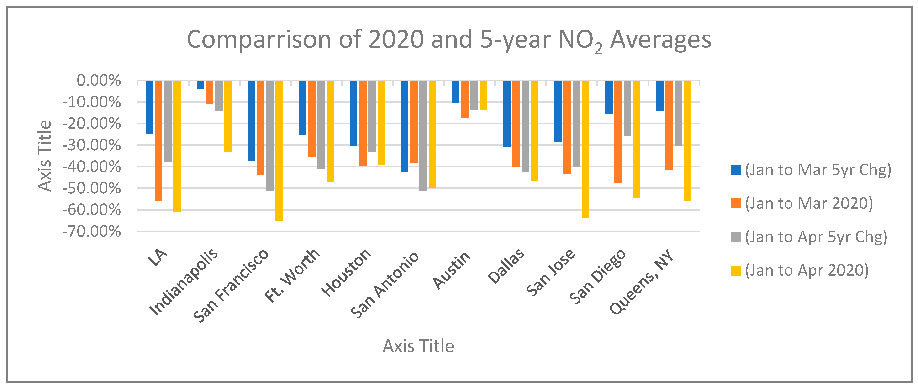
The percentage drop in NO2 values when 2020 values are compared to the 5-year averages between January and March range from 11–56% and 4–43%, respectively (Table 1 and Table 2), while January and April reflect a NO2 drop ranging from 14–65% in 2020 and a drop of 13–51% in the 5-year averages (Table 1 and Table 2). Between January and March, San Antonio was the only location where the 2020 percent change was lower than the 5-year average percent change (Figure 1). From January to April (Figure 1), the percent changes in 2020 and the 5-year averages of San Antonio and Austin were almost the same, while the other nine locations showed a sharp reduction in NO2 values in 2020 compared to the same 2-month window from 2015–2019 (Figure 1). Excluding the cities of Austin and San Antonio from January to April in 2020, Indianapolis had the smallest reduction of NO2 at 33%, and San Francisco had the largest reduction of NO2 values at 65% (Table 1).
Seasonal changes in NO2 naturally occur and must be considered. In summer, NOx and other volatile organic compounds from traffic and other sources result in photochemical smog, with December through February having seasonal maximum in the U.S. [31]. Oxidation by photochemically produced OH in the summer reduces NOx, while lower concentrations of OH in the winter months results in an increased lifetime of NOx [32]. Extrapolating further from Table 1, we see this in our multi-city data, with an average decrease in 2020 NO2 values in March and April ranging from −40% to −50% compared to their respective average January values. In April 2020, Austin had the smallest reduction of −13.51%, with San Francisco having the largest reduction of −64.93% (Table 1). These decreases constitute seasonal changes plus any change related to COVID lockdown policies in the various cities.
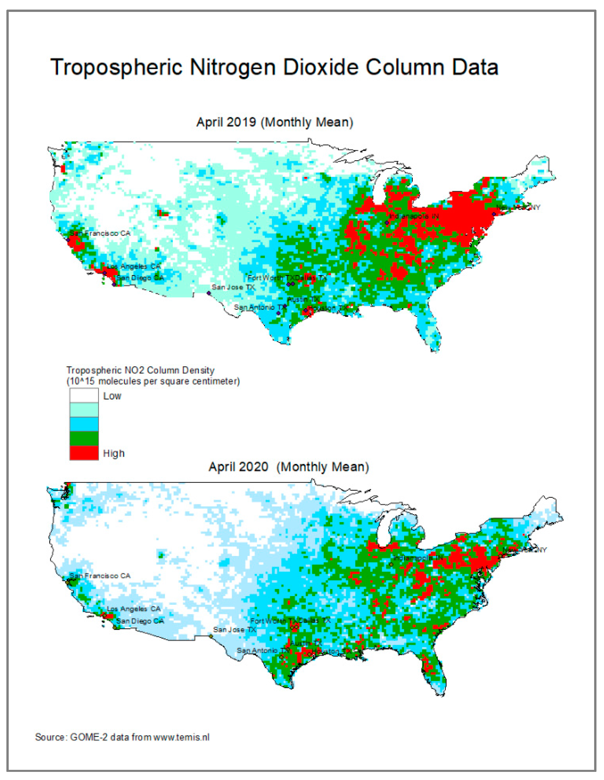
To determine the typical seasonal decrease in NO2 values and thus remove this from the COVID-related signals, we calculated the 5-year averages for each city to normalize for weather-related variations year-on-year. We found that the typical seasonal decreases were significantly less than the COVID-impacted 2020 decreases (Figure 1). With the exception of Ft. Worth, San Antonio, and Dallas, rest of the cities had a greater than 20% drop in March–April averages in 2020 versus the 5-year averages (Figure 2). On average, between January and March and January and April in 2020, NO2 values decreased by 14% when compared to their respective 5-year averages from 2015–2019 (Table 1 and Table 2), indicating the significant impact of lockdowns and agreeing with the more regional results obtained by satellite analysis [33]. We can visualize such impacts from the free use of tropospheric NO2 monthly mean averages from GOME-2 sensor from www.temis.nl over the U.S. from April 2019 when compared to April 2020 (Figure 3) [34].
3.2. VMT and NO2
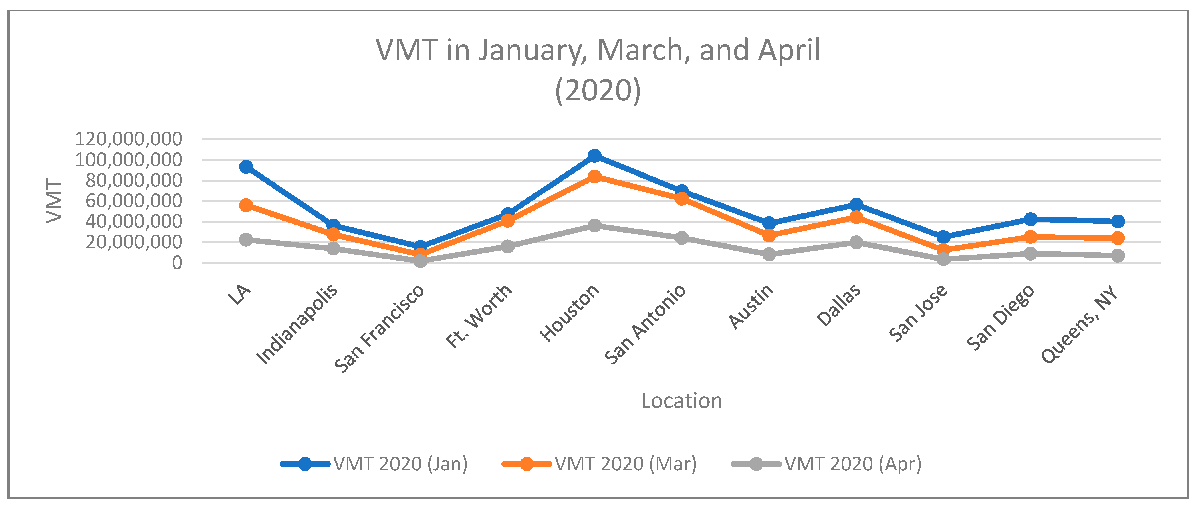
Similar to the NO2 trends between January, March, and April in 2020 (Figure 4), VMT in all the locations significantly dropped with the implementation of stay-at-home orders (Figure 5). March showed a significant reduction in VMT between 11–51%, with NO2 reduction being between 11–56% (Table 3). April in comparison to January showed a much higher reduction of VMT between 62–89% (Table 3), with NO2 reduction being between 14–65% (Table 3, Figure 6).
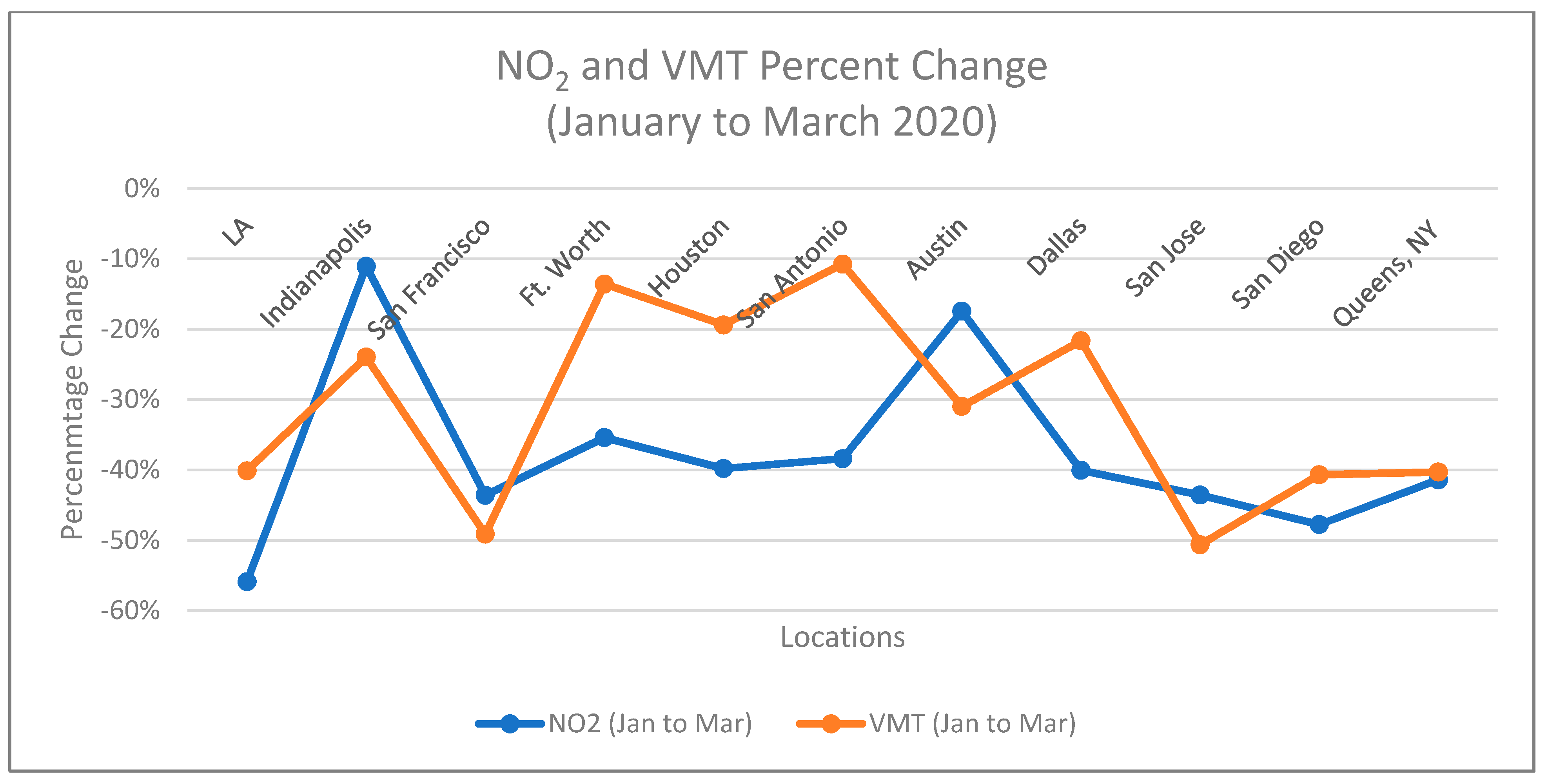
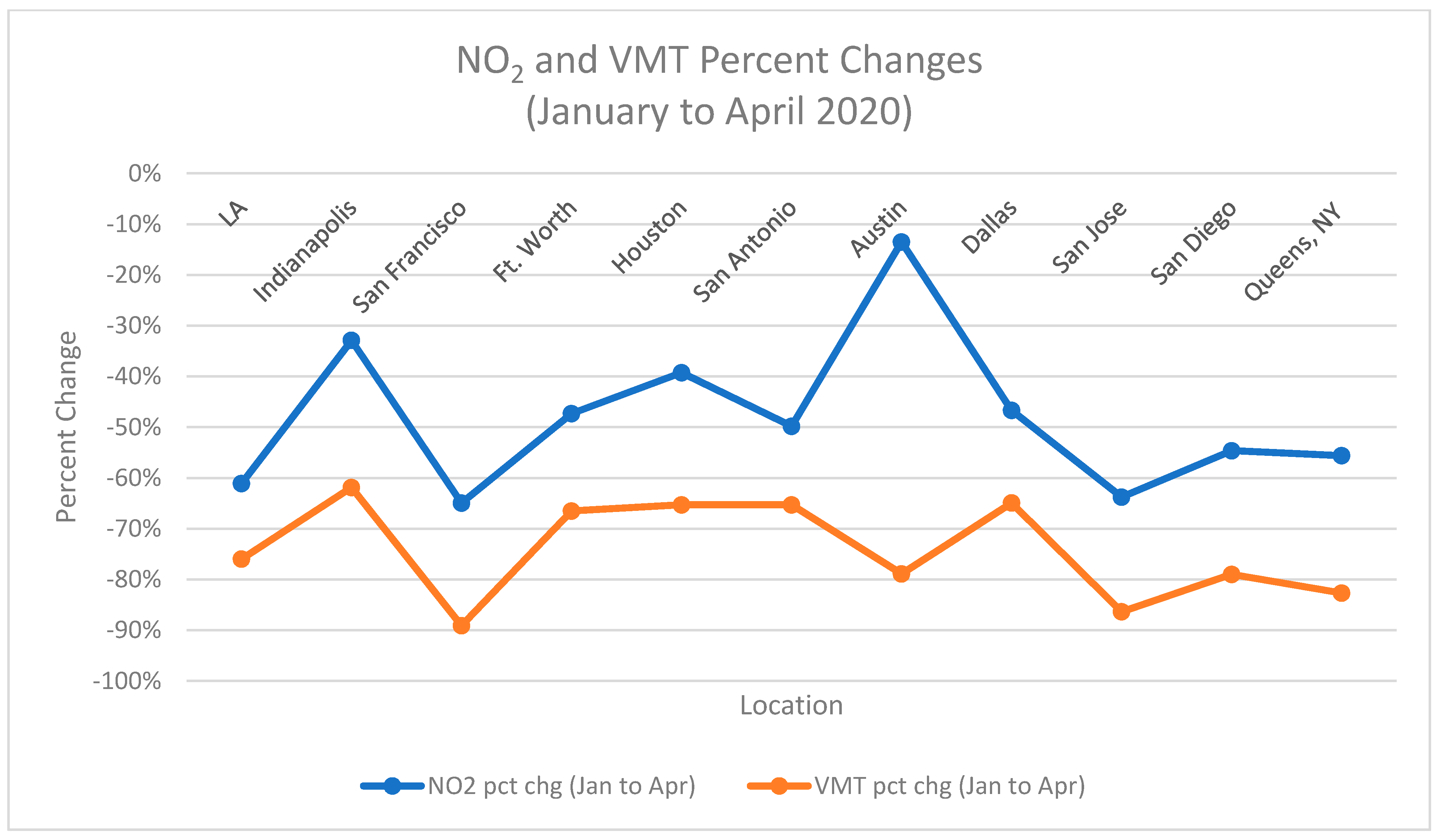
Comparing the trends of NO2 and VMT from January to March 2020, the percentage changes of NO2 of Indianapolis, San Francisco, Austin, and San Jose are higher than the VMT percent changes in the same time frame. For LA, Ft Worth, Houston, San Antonio, Dallas, and San Diego, VMT percent changes, causes of which were not investigated, are lower than the NO2 percent changes, with Queens being about the same (Figure 7). For April, a month into the shutdown period in most states, NO2 changes are consistently higher than the VMT percent changes in that time (Figure 8).
Spearman rank-correlation statistics was calculated between NO2 and VMT, with alpha level set at 0.05 to examine the strength of their relationship. It ranges between −1 to +1, with zero indicating no association between two variables; −1 indicating a perfectly inverse strength of relationship; and a +1 indicating a perfect strength of association. This analysis revealed that San Diego, San Jose, and Indianapolis have higher significant correlation (r = 0.43–0.53) and LA, Houston, San Francisco, and Queens have lower significant correlations (r = 0.29–0.39) (Table 4). High p-values for the four cities in Texas (Ft. Worth, San Antonio, Austin, and Dallas) indicate that, in those locations, we do not have strong evidence of a relationship between NO2 and VMT variations, thus preventing us from understanding the relationship with this dataset. Examining the ratios of NO2 to VMT for January to April 2020 for all 11 cities, we find that, on average, a 1,000,000 reduction in VMT resulted in a reduction of 0.24 ppb in NO2 for all cities. Austin was well below that average, at 0.06 ppb, and San Francisco had the highest impact of the decreased VMT (with a reduction of 0.65 ppb) for an average of a 1,000,000 reduction in VMT (Table 5).
3.3. Indianapolis Road Sensor Data
Given that the Spearman correlation between NO2 and VMT in Indianapolis is significant, we examined the city further. An expanded Spearman correlation test indicates that the correlation between VMT, NO2, and vehicle counts in March and April 2020 are all highly significant, with moderate correlations between VMT and NO2 and high correlations between total vehicles and VMT, as expected (Table 6).
Average counts of total vehicles, vehicle classification excluding categories 1–4 (excluding motorcycle, car, pickup, and bus—proxy for trucks), NO2, and VMT show a decline in all categories in March and April when compared to January 2020 (Table 7). VMT percentage reduction in April versus January is almost two times that of the average total vehicles in Indianapolis and of the NO2 percentage reduction in that time period (Table 8), indicating that a percentage reduction in the average total vehicles results in almost an equivalent percentage reduction in NO2 in the city in that month. Extrapolating from Table 8, we can make the following observation regarding the change from January to April:
An average of 1876 (38,494–36,618)-unit reduction in average total vehicles, excluding motorcycle, car, pickup, and bus, is equivalent to a 32% [35] or an 1.11 ppb (0.32 × 3.46) average burden reduction of NO2 in Indianapolis.
4. Discussion
The onset of COVID-19 and the stay-at-home orders in March and April have presented an opportunity to examine the changes in NO2 concentrations and their relationship to VMT in 11 cities in the U.S., with implications for local health outcomes.
Our analysis of the impacts of stay-at-home orders utilized ground-based sensor data from 11 U.S. cities. We found an average reduction of NO2 of 45% measured in March and April 2020 when compared with their 5-year averages of 29% (2015–2019) (Table 1 and Table 2). January to April 2020 resulted in a NO2 drop between 14–65% versus its respective 5-year average drop between 13–51%. Four Texas cities had poor correlation between VMT and NO2 (Ft. Worth, San Antonio, Austin, and Dallas). This offset compared to studies using satellite data is likely due to differences in the air being sampled with each approach (i.e., ground-level versus troposphere scale). San Diego, San Jose, and Indianapolis had the strongest strength of relationship between VMT and NO2, as is illustrated from the correlation analysis.
The VMT reduction in April 2020 ranged between 62% and 89% (Table 3) when compared to January 2020. Average ratios of NO2/VMT for the 11 locations indicates that for every 1,000,000 less VMT, NO2 decreases by an average of 0.24 ppb (Table 5). A 1,000,000 average VMT drop in San Francisco resulted in the most significant decrease in NO2 (0.65 ppb), and Houston resulted in the least significant decrease (0.07 ppb). The petrochemical industry in Texas, and particularly in the greater Houston area, probably plays a significant role in NO2 production [36], and thus the VMT-NO2 relationship is not likely the only significant factor influencing the scale of observed decreases in NO2.
The lack of observed significant correlations between NO2 and VMT for the four Texas cities remains unresolved. We suggest two options: (1) the locations of the fixed AQ sensors’ locations in relation to emission sources as related to traffic and non-traffic need to be identified and incorporated with meteorology, as their absence may not be ideal for capturing the more regional emission sources that are better characterized by satellite observations [33] that might be an issue for more sprawling cities, and/or (2) VMT along with specific traffic volume and classification analysis from platforms like StreetLight may be a more robust metric for extrapolating local impacts of NO2 emissions from vehicle sources. A much denser array of high-quality, ground-based sensors would likely have to be in place to address option (1) above, but with option (2), we can, at least for one of the cities (Indianapolis), compare NO2 to actual vehicle count and classification data for several locations to address the issue.
Since VMT may not be the best indicator of pollution impacts, we can use traffic counts and vehicle classifications in addition to VMT to create localized indices that can assist local governments to plan and/or to adjust traffic flows to address the impacts of high NO2 values. In future studies, placement of NO2 sensors in relation to the NO2 sources, which would also impact the sensors readings, should be considered. This NO2/VMT ratio (Table 5) should be tested in other cities in different seasons, which could be then used as a proxy in examining NO2 production in different regions while gauging the impact of transportation changes. This can assist in classifying the impact of traffic changes in regions from the most sensitive to the least. In addition to sensor placement, meteorological conditions, like temperature, wind speed, relative humidity, and precipitation, also play a role in the transport of atmospheric gases [37], which were also not considered in this analysis. Such conditions are not uniform spatially and have shown to cause column NO2 readings to differ by about 15% over monthly timescales [33]; high winds in particular can play a role in dispersing NO2 pollutant concentrations throughout the year [38].
A deeper look into vehicle counts and classification in Indianapolis indicates that the drop in average total vehicles percentage is almost identical to the percentage drop in its NO2 values (Table 8). An 1876-unit reduction in proxy truck average in Indianapolis results in lowering VMT, which in turn should yield a decrease in average NO2 values by 1.11 ppb (Table 8). Building on this process in time and space, this calculation can be useful in examining regions that should be targeted first and would have the biggest impact of the reduction in NO2 through traffic manipulation. In places like Houston, where there is a presence of other significant industrial emissions of NO2, their emission impacts should also be incorporated for a more comprehensive understanding.
In qualitative terms, the observed substantial reductions in NO2 would, all other things being equal, provide some benefits to human health. With the return to business-as-usual practices, these health benefits will be transitory. Satellite measurements of NO2 are outstanding for capturing regional trends, but the heterogeneity of NO2 at the ground level in a given city [39] is not well-captured and thus pinpointing that emission sources that are proximal to population centers at the fine scale should be a high priority for city planners and transportation design. This latter point is critical in that the highest concentrations of NO2 and many other criteria air pollutants are disproportionately located in lower-income communities [25,40]. The overlapping issues of poor air quality and particular susceptibility, likely via co-morbidities, of these same communities to severe COVID disease [41] speaks to the need to better constrain ground-level air pollution levels with an eye toward applying health equity solutions in cities.
5. Conclusions
The pandemic-driven shutdown policies instituted in cities across the U.S. substantially decreased many harmful air pollutants, including NO2 [33,42]. We found this stable reduction within cities using ground-based monitors, and it is largely tied to reduced traffic volume, with other factors, such as industrial emissions, playing a variable role. Although ground-based monitoring ties the concentration data much more closely to communities and local health impacts than does more regionally comprehensive satellite data, the paucity of monitors and likely disconnects between metrics that are meant to capture traffic volume reduces their effectiveness from a public health standpoint.
This observed reduction in urban NO2 concentrations ranging between 11% and 65%, a rare silver lining of the devastating pandemic, is likely temporary, but it does point to the tight connection between traffic-related pollution sources and local impacts. This connection highlights a two-fold issue: that local air-pollution hotspots may exacerbate diseases like COVID and are currently under-studied, especially when it comes to examining pollutant burden by taking vehicle classifications into account, as we illustrated in Indianapolis, where we accounted for an average of 1.11 ppb reduction in NO2. Two actions that city planners can take to promote health equity in their communities are to implement environmental-monitoring programs that link data points (i.e., monitors) more strategically to population density and to implement local transportation and zoning policies that examine and protect community health and build health equity into the system.
Author Contributions
Conceptualization, data curation, analysis, writing, and editing, A.H.; conceptualization and writing, G.F.; conceptualization and writing, V.L. All authors have read and agreed to the published version of the manuscript.
Funding
This work was partially supported by the Environmental Resilience Institute, funded by Indiana University’s Prepared for Environmental Change Grand Challenge Initiative and by National Science Foundation award ICER-1701132 to Filippelli. The source data for NO2 concentrations were accessed from the public databases available at the Department of Environmental Management or equivalent data hubs for each state. The VMT data, an unfunded aspect of this project, can be accessed at the Streetlight data hub (https://www.streetlightdata.com, 15 May 2020). The vehicle-count data for the city of Indianapolis can be accessed at the Indiana Department of Transportation site (www.indot.in.gov, 18 November 2020).
Data Availability Statement
Data sharing not applicable.
Conflicts of Interest
The authors declare no conflict of interest.
References
- WHO Director-General’s Opening Remarks at the Media Briefing on COVID-19 - 11 March 2020. Available online: https://www.who.int/dg/speeches/detail/who-director-general-s-opening-remarks-at-the-media-briefing-on-covid-19---11-march-2020 (accessed on 21 May 2020).
- CDC COVID Data Tracker. Available online: https://www.cdc.gov/covid-data-tracker/#cases (accessed on 12 August 2020).
- Nakada, L.Y.K.; Urban, R.C. COVID-19 Pandemic: Impacts on the Air Quality during the Partial Lockdown in São Paulo State, Brazil. Sci. Total Environ. 2020, 730, 139087. [Google Scholar] [CrossRef] [PubMed]
- Sharma, S.; Zhang, M.; Anshika; Gao, J.; Zhang, H.; Kota, S.H. Effect of Restricted Emissions during COVID-19 on Air Quality in India. Sci. Total Environ. 2020, 728, 138878. [Google Scholar] [CrossRef]
- Tanzer-Gruener, R.; Li, J.; Eilenberg, S.R.; Robinson, A.L.; Presto, A.A. Impacts of Modifiable Factors on Ambient Air Pollution: A Case Study of COVID-19 Shutdowns. Environ. Sci. Technol. Lett. 2020, 7, 554–559. [Google Scholar] [CrossRef]
- Şahin, Ü.A. The Effects of COVID-19 Measures on Air Pollutant Concentrations at Urban and Traffic Sites in Istanbul. Aerosol Air Qual. Res. 2020, 20, 1874–1885. [Google Scholar] [CrossRef]
- Wu, C.; Wang, H.; Cai, W.; He, H.; Ni, A.; Peng, Z. Impact of the COVID-19 Lockdown on Roadside Traffic-Related Air Pollution in Shanghai, China. Build. Environ. 2021, 194, 107718. [Google Scholar] [CrossRef]
- Baldasano, J.M. COVID-19 Lockdown Effects on Air Quality by NO2 in the Cities of Barcelona and Madrid (Spain). Sci. Total Environ. 2020, 741, 140353. [Google Scholar] [CrossRef]
- Bauwens, M.; Compernolle, S.; Stavrakou, T.; Müller, J.-F.; Gent, J.; van Eskes, H.; Levelt, P.F.; van der A, R.; Veefkind, J.P.; Vlietinck, J.; et al. Impact of Coronavirus Outbreak on NO2 Pollution Assessed Using TROPOMI and OMI Observations. Geophys. Res. Lett. 2020, 47, e2020GL087978. [Google Scholar] [CrossRef]
- Lamsal, L.; Krotkov, N.; Celarier, E.; Swartz, W.; Pickering, K.; Bucsela, E.; Gleason, J.; Martin, R.; Philip, S.; Irie, H.; et al. Evaluation of OMI Operational Standard NO2 Retrievals Using in Situ and Surface-Based NO2 Observations. Atmos. Chem. Phys. 2014, 14, 11587–11609. [Google Scholar] [CrossRef] [Green Version]
- Walters, W.W.; Goodwin, S.R.; Michalski, G. Nitrogen Stable Isotope Composition (Δ15N) of Vehicle-Emitted NOx. Environ. Sci. Technol. 2015, 49, 2278–2285. [Google Scholar] [CrossRef]
- Jaeglé, L.; Steinberger, L.; Martin, R.V.; Chance, K. Global Partitioning of NOx Sources Using Satellite Observations: Relative Roles of Fossil Fuel Combustion, Biomass Burning and Soil Emissions. Faraday Discuss. 2005, 130, 407–423. [Google Scholar] [CrossRef] [PubMed]
- Cesaroni, G.; Badaloni, C.; Gariazzo, C.; Stafoggia, M.; Sozzi, R.; Davoli, M.; Forastiere, F. Long-Term Exposure to Urban Air Pollution and Mortality in a Cohort of More than a Million Adults in Rome. Environ. Health Perspect. 2013, 121, 324–331. [Google Scholar] [CrossRef] [PubMed] [Green Version]
- Peel, J.L.; Tolbert, P.E.; Klein, M.; Metzger, K.B.; Flanders, W.D.; Todd, K.; Mulholland, J.A.; Ryan, P.B.; Frumkin, H. Ambient Air Pollution and Respiratory Emergency Department Visits. Epidemiology 2005, 16, 164–174. [Google Scholar] [CrossRef]
- Bermejo-Orduna, R.; McBride, J.R.; Shiraishi, K.; Elustondo, D.; Lasheras, E.; Santamaría, J.M. Biomonitoring of Traffic-Related Nitrogen Pollution Using Letharia Vulpina (L.) Hue in the Sierra Nevada, California. Sci. Total Environ. 2014, 490, 205–212. [Google Scholar] [CrossRef]
- Galloway, J.N.; Aber, J.D.; Erisman, J.W.; Seitzinger, S.P.; Howarth, R.W.; Cowling, E.B.; Cosby, B.J. The Nitrogen Cascade. BioScience 2003, 53, 341–356. [Google Scholar] [CrossRef]
- Marco, R.D.; Poli, A.; Ferrari, M.; Accordini, S.; Giammanco, G.; Bugiani, M.; Villani, S.; Ponzio, M.; Bono, R.; Carrozzi, L.; et al. The Impact of Climate and Traffic-Related NO2 on the Prevalence of Asthma and Allergic Rhinitis in Italy. Clin. Exp. Allergy 2002, 32, 1405–1412. [Google Scholar] [CrossRef] [PubMed]
- Redling, K.; Elliott, E.; Bain, D.; Sherwell, J. Highway Contributions to Reactive Nitrogen Deposition: Tracing the Fate of Vehicular NO x Using Stable Isotopes and Plant Biomonitors. Biogeochemistry 2013, 116, 261–274. [Google Scholar] [CrossRef]
- Achakulwisut, P.; Brauer, M.; Hystad, P.; Anenberg, S.C. Global, National, and Urban Burdens of Paediatric Asthma Incidence Attributable to Ambient NO2 Pollution: Estimates from Global Datasets. Lancet Planet. Health 2019, 3, e166–e178. [Google Scholar] [CrossRef] [Green Version]
- New York State Air Quality. Available online: http://www.nyaqinow.net/ (accessed on 1 July 2021).
- Quality Assurance Air Monitoring Site Information | California Air Resources Board. Available online: https://ww2.arb.ca.gov/applications/quality-assurance-air-monitoring-site-information (accessed on 1 July 2021).
- GeoTAM. Available online: https://tceq.maps.arcgis.com/apps/webappviewer/index.html?id=ab6f85198bda483a997a6956a8486539 (accessed on 1 July 2021).
- Daily Summary Report By Site. Available online: https://idem.meteostar.com/cgi-bin/select_summary.pl (accessed on 1 July 2021).
- Air Sensor Guidebook. Available online: https://cfpub.epa.gov/si/si_public_file_download.cfm?p_download_id=519616 (accessed on 1 July 2021).
- Cakmak, S.; Hebbern, C.; Cakmak, J.D.; Vanos, J. The Modifying Effect of Socioeconomic Status on the Relationship between Traffic, Air Pollution and Respiratory Health in Elementary Schoolchildren. J. Environ. Manag. 2016, 177, 1–8. [Google Scholar] [CrossRef] [Green Version]
- Jia, C.; Fu, X.; Bartelli, D.; Smith, L. Insignificant Impact of the “Stay-At-Home” Order on Ambient Air Quality in the Memphis Metropolitan Area, U.S.A. Atmosphere 2020, 11, 630. [Google Scholar] [CrossRef]
- StreetLight Volume Methodology & Validation White Paper. Available online: https://www.streetlightdata.com/ (accessed on 1 July 2021).
- Madariaga, I.; Agirre, E.; Uria, J. Short-Term Forecasting of Ozone and NO2 levels Using Traffic Data in Bilbao (Spain). WIT Trans. Built Environ. 2003, 64, 8. [Google Scholar]
- Nicolai, T.; Carr, D.; Weiland, S.K.; Duhme, H.; von Ehrenstein, O.; Wagner, C.; von Mutius, E. Urban Traffic and Pollutant Exposure Related to Respiratory Outcomes and Atopy in a Large Sample of Children. Eur Respir J. 2003, 21, 956–963. [Google Scholar] [CrossRef] [PubMed] [Green Version]
- Traffic Count Database System (TCDS). Available online: https://indot.ms2soft.com/tcds/tsearch.asp?loc=indot (accessed on 13 August 2020).
- van der A, R.J.; Eskes, H.J.; Boersma, K.F.; Noije, T.P.C.; van Roozendael, M.V.; Smedt, I.D.; Peters, D.H.M.U.; Meijer, E.W. Trends, Seasonal Variability and Dominant NOx Source Derived from a Ten Year Record of NO2 Measured from Space. J. Geophys. Res. Atmos. 2008, 113. [Google Scholar] [CrossRef]
- Shah, V.; Jacob, D.J.; Li, K.; Silvern, R.F.; Zhai, S.; Liu, M.; Lin, J.; Zhang, Q. Effect of Changing NOx Lifetime on the Seasonality and Long-Term Trends of Satellite-Observed Tropospheric NO2 Columns over China. Atmos. Chem. Phys. 2020, 20, 1483–1495. [Google Scholar] [CrossRef] [Green Version]
- Goldberg, D.L.; Anenberg, S.C.; Griffin, D.; McLinden, C.A.; Lu, Z.; Streets, D.G. Disentangling the Impact of the COVID-19 Lockdowns on Urban NO2 From Natural Variability. Geophys. Res. Lett. 2020, 47, e2020GL089269. [Google Scholar] [CrossRef]
- Boersma, K.F.; Eskes, H.J.; Brinksma, E.J. Error Analysis for Tropospheric NO2 Retrieval from Space. J. Geophys. Res. Atmos. 2004, 109. [Google Scholar] [CrossRef]
- Matthes, S.; Grewe, V.; Sausen, R. Global Impact of Road Traffic Emissions on Tropospheric Ozone. Atmos. Chem. Phys. 2007, 7, 1707–1718. [Google Scholar] [CrossRef] [Green Version]
- Jobson, B.T.; Berkowitz, C.M.; Kuster, W.C.; Goldan, P.D.; Williams, E.J.; Fesenfeld, F.C.; Apel, E.C.; Karl, T.; Lonneman, W.A.; Riemer, D. Hydrocarbon Source Signatures in Houston, Texas: Influence of the Petrochemical Industry. J. Geophys. Res. Atmos. 2004, 109. [Google Scholar] [CrossRef]
- Tobías, A.; Carnerero, C.; Reche, C.; Massagué, J.; Via, M.; Minguillón, M.C.; Alastuey, A.; Querol, X. Changes in Air Quality during the Lockdown in Barcelona (Spain) One Month into the SARS-CoV-2 Epidemic. Sci. Total Environ. 2020, 726, 138540. [Google Scholar] [CrossRef]
- Arain, M.A.; Blair, R.; Finkelstein, N.; Brook, J.; Jerrett, M. Meteorological Influences on the Spatial and Temporal Variability of NO2 in Toronto and Hamilton. Can. Geogr./Le Géographe Can. 2009, 53, 165–190. [Google Scholar] [CrossRef]
- Coppalle, A.; Delmas, V.; Bobbia, M. Variability of Nox and No2 Concentrations Observed at Pedestrian Level in the City Centre of a Medium Sized Urban Area. Atmos. Environ. 2001, 35, 5361–5369. [Google Scholar] [CrossRef]
- Miranda, M.L.; Edwards, S.E.; Keating, M.H.; Paul, C.J. Making the Environmental Justice Grade: The Relative Burden of Air Pollution Exposure in the United States. Int. J. Environ. Res. Public Health 2011, 8, 1755–1771. [Google Scholar] [CrossRef] [PubMed]
- Fattorini, D.; Regoli, F. Role of the Chronic Air Pollution Levels in the Covid-19 Outbreak Risk in Italy. Environ. Pollut 2020, 264, 114732. [Google Scholar] [CrossRef]
- Berman, J.D.; Ebisu, K. Changes in U.S. Air Pollution during the COVID-19 Pandemic. Sci Total Environ. 2020, 739, 139864. [Google Scholar] [CrossRef] [PubMed]
Figure 1.
January to March and January to April NO2 changes for 2020, the average of the previous 5-years of non-COVID conditions, and the decrease from annual averages.
Figure 1.
January to March and January to April NO2 changes for 2020, the average of the previous 5-years of non-COVID conditions, and the decrease from annual averages.

Figure 2.
March and April combined NO2 averages in parts per billion (ppb) from 2020 versus 5 -year (2015-2019).
Figure 2.
March and April combined NO2 averages in parts per billion (ppb) from 2020 versus 5 -year (2015-2019).

Figure 3.
NO2 averages from April in 2019 and 2020.

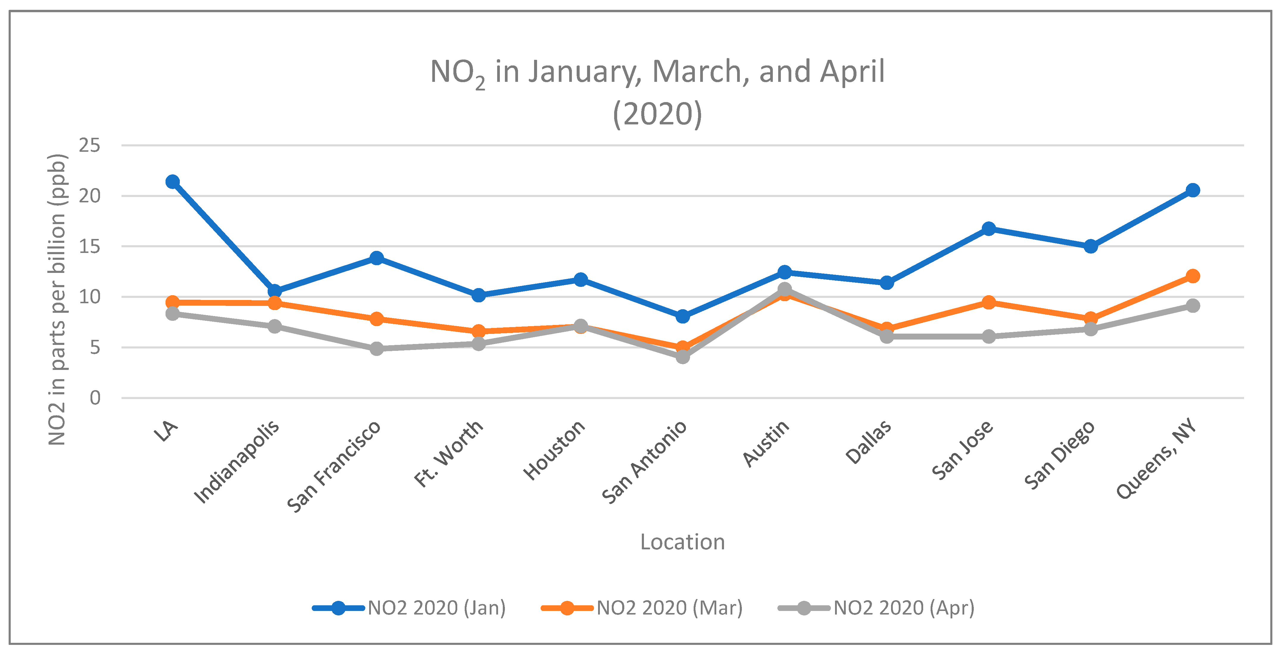
Figure 4.
NO2 averages from January, March, and April in 2020.

Figure 5.
Vehicle miles travelled (VMT) for 11 cities from January, March, and April of 2020.

Figure 6.
VMT changes between January to March and January to April in 2020.

Figure 7.
NO2 and VMT percent changes between January and March in 2020.

Figure 8.
NO2 and VMT percent changes between January and April 2020.


Table 1.
2020 NO2 averages and percent changes in 2020.
| Location (NO2 Sensors) | Jan (ppb) | Mar (ppb) | Apr (ppb) | 2020 Change (Jan to Mar) | 2020 Change (Jan to Apr) |
|---|---|---|---|---|---|
| LA | 21.40 | 9.44 | 8.33 | −55.89% | −61.08% |
| Indianapolis | 10.54 | 9.38 | 7.08 | −11.03% | −32.90% |
| San Francisco | 13.84 | 7.81 | 4.85 | −43.59% | −64.93% |
| Ft. Worth | 10.15 | 6.56 | 5.35 | −35.39% | −47.32% |
| Houston | 11.70 | 7.04 | 7.11 | −39.79% | −39.25% |
| San Antonio | 8.06 | 4.96 | 4.04 | −38.39% | −49.82% |
| Austin | 12.43 | 10.26 | 10.75 | −17.42% | −13.51% |
| Dallas | 11.38 | 6.82 | 6.07 | −40.05% | −46.67% |
| San Jose | 16.74 | 9.45 | 6.07 | −43.55% | −63.76% |
| San Diego | 14.99 | 7.83 | 6.80 | −47.76% | −54.62% |
| Queens, NY | 20.55 | 12.04 | 9.12 | −41.39% | −55.61% |
Table 2.
NO2 averages of January, March, and April from 2015–2019.
| Location (NO2 Sensors) | Jan (ppb) | Mar (ppb) | Apr (ppb) | 5-yr Change (Jan to Mar) | 5-yr Change (Jan to Apr) |
|---|---|---|---|---|---|
| LA | 22.01 | 16.60 | 13.68 | −24.57% | −37.85% |
| Indianapolis | 13.79 | 13.23 | 11.83 | −4.00% | −14.18% |
| San Francisco | 18.21 | 11.45 | 8.88 | −37.12% | −51.21% |
| Ft. Worth | 10.26 | 7.69 | 6.07 | −25.09% | −40.88% |
| Houston | 15.00 | 10.42 | 10.02 | −30.54% | −33.20% |
| San Antonio | 9.64 | 5.54 | 4.71 | −42.56% | −51.10% |
| Austin | 15.42 | 13.83 | 13.35 | −10.32% | −13.44% |
| Dallas | 12.57 | 8.73 | 7.25 | −30.61% | −42.34% |
| San Jose | 18.11 | 12.98 | 10.80 | −28.31% | −40.38% |
| San Diego | 15.32 | 12.93 | 11.41 | −15.64% | −25.51% |
| Queens, NY | 20.60 | 17.68 | 14.35 | −14.14% | −30.31% |
Table 3.
NO2 and VMT changes between January to March and January to April 2020.
| Location | NO2 Jan to Mar | VMT Jan to Mar | NO2 Jan to Apr | VMT Jan to Apr |
|---|---|---|---|---|
| LA | −55.89% | −40.11% | −61.08% | −75.97% |
| Indianapolis | −11.03% | −23.95% | −32.90% | −61.87% |
| San Francisco | −43.59% | −49.12% | −64.93% | −89.07% |
| Ft. Worth | −35.39% | −13.57% | −47.32% | −66.50% |
| Houston | −39.79% | −19.38% | −39.25% | −65.29% |
| San Antonio | −38.39% | −10.73% | −49.82% | −65.29% |
| Austin | −17.42% | −30.97% | −13.51% | −78.88% |
| Dallas | −40.05% | −21.63% | −46.67% | −64.91% |
| San Jose | −43.55% | −50.62% | −63.76% | −86.35% |
| San Diego | −47.76% | −40.69% | −54.62% | −78.99% |
| Queens, NY | −41.39% | −40.29% | −55.61% | −82.66% |
Table 4.
Spearman correlations between NO2 and VMT in March and April of 2020 (alpha = 0.05).
| Location | X | Y | Correlation Coefficient | p-Value | p-Value < 0.05 |
|---|---|---|---|---|---|
| LA | NO2 | VMT | 0.3543 | 0.0051 | X |
| Indianapolis | NO2 | VMT | 0.4569 | 0.0002 | X |
| San Francisco | NO2 | VMT | 0.3230 | 0.0111 | X |
| Ft Worth | NO2 | VMT | 0.1329 | 0.3072 | |
| Houston | NO2 | VMT | 0.2910 | 0.0229 | X |
| San Antonio | NO2 | VMT | 0.2225 | 0.0848 | |
| Austin | NO2 | VMT | 0.0454 | 0.7285 | |
| Dallas | NO2 | VMT | 0.1173 | 0.3679 | |
| San Jose | NO2 | VMT | 0.4295 | 0.0006 | X |
| San Diego | NO2 | VMT | 0.5320 | 0.0000 | X |
| Queens | NO2 | VMT | 0.3916 | 0.0028 | X |
Table 5.
NO2 and VMT ratios from January to April 2020 for cities.
| Location | VMT Avg Chg (Jan–Apr) = [B] | NO2 Avg Chg in ppb (Jan–Apr) = [A] | NO2/VMT = A/B (all Cities) |
|---|---|---|---|
| LA | −70,802,793.41 | −13.07 | 0.18 × 10⁻⁶ |
| Indianapolis | −22,364,196.21 | −3.47 | 0.16 × 10⁻⁶ |
| San Francisco | −13,824,506.67 | −8.99 | 0.65 × 10⁻⁶ |
| Ft. Worth | −31,308,793.60 | −4.80 | 0.15 × 10⁻⁶ |
| Houston | −67,843,483.92 | −4.59 | 0.07 × 10⁻⁶ |
| San Antonio | −45,369,086.33 | −4.01 | 0.09 × 10⁻⁶ |
| Austin | −30,210,481.83 | −1.68 | 0.06 × 10⁻⁶ |
| Dallas | −36,617,918.66 | −5.31 | 0.15 × 10⁻⁶ |
| San Jose | −21,531,553.94 | −10.67 | 0.50 × 10⁻⁶ |
| San Diego | −33,359,270.66 | −8.19 | 0.25 × 10⁻⁶ |
| Queens | −33,089,110.33 | −11.43 | 0.35 × 10⁻⁶ |
| Average | 0.24 × 10⁻⁶ |
Table 6.
Spearman correlation between vehicles and VMT and NO2 in Indianapolis, March–April 2020.
| Location | X | Y | Correlation Coefficient | p-Value |
|---|---|---|---|---|
| Indianapolis | Avg Total Vehicles | VMT | 0.90 | <0.005 |
| Indianapolis | Avg Total Vehicles | NO2 | 0.54 | <0.005 |
| Indianapolis | VMT | NO2 | 0.46 | <0.006 |
Table 7.
Indianapolis vehicle count, NO2, and VMT in 2020.
| Month | Avg Total Vehicles | Avg Total Cars | Avg Vehicles (1 to 4) | Avg Vehicles (Excl 1 to 4) | Avg NO2 2020 (ppb) | Avg VMT 2020 |
|---|---|---|---|---|---|---|
| Jan | 336,971 | 239,289 | 298,476 | 38,494 | 10.54 | 36,147,631 |
| Mar | 310,327 | 210,699 | 268,216 | 42,111 | 9.38 | 27,490,875 |
| Apr | 220,784 | 137,125 | 184,166 | 36,618 | 7.08 | 13,783,435 |
Table 8.
Percentage and unit change of vehicles, VMT, and NO2 from January to April to January 2020.
Table 8.
Percentage and unit change of vehicles, VMT, and NO2 from January to April to January 2020.
| Variable | January | April | Unit_Chg (Jan–April) | Pct_Chg (Jan–Apr) |
|---|---|---|---|---|
| Avg_VMT | 36,147,631 | 13,783,435 | −22,364,196 | −61.87% |
| Avg_NO2(ppb) 1 | 10.54 | 7.08 | −3.46 | −32.83% |
| Avg_tot_veh 2 | 336,971 | 220,784 | 116,187 | −34.48% |
| Avg_tot_cars 3 | 239,289 | 137,125 | 102,164 | −42.69% |
| Avg_veh (1–4) 4 | 298,476 | 184,166 | 114,310 | −38.30% |
| Avg_veh (excl 1–4) 5 | 38,494 | 36,618 | 1876 | −4.87% |
1 NO2 averaged from two sensors in Indianapolis. 2 Total count of vehicles averaged over the 5 sensors in Indianapolis. 3 Total count of cars averaged over the 5 sensors in Indianapolis. 4 Total count of vehicle class 1–4 (motorcycle, car, pickup, and bus) averaged over the 5 sensors in Indianapolis. 5 Total count of a proxy for trucks averaged over the 5 sensors in Indianapolis.
Publisher’s Note: MDPI stays neutral with regard to jurisdictional claims in published maps and institutional affiliations. |
© 2021 by the authors. Licensee MDPI, Basel, Switzerland. This article is an open access article distributed under the terms and conditions of the Creative Commons Attribution (CC BY) license (https://creativecommons.org/licenses/by/4.0/).
Share and Cite
MDPI and ACS Style
Heintzelman, A.; Filippelli, G.; Lulla, V. Substantial Decreases in U.S. Cities’ Ground-Based NO2 Concentrations during COVID-19 from Reduced Transportation. Sustainability 2021, 13, 9030. https://doi.org/10.3390/su13169030
AMA Style
Heintzelman A, Filippelli G, Lulla V. Substantial Decreases in U.S. Cities’ Ground-Based NO2 Concentrations during COVID-19 from Reduced Transportation. Sustainability. 2021; 13(16):9030. https://doi.org/10.3390/su13169030
Chicago/Turabian StyleHeintzelman, Asrah, Gabriel Filippelli, and Vijay Lulla. 2021. "Substantial Decreases in U.S. Cities’ Ground-Based NO2 Concentrations during COVID-19 from Reduced Transportation" Sustainability 13, no. 16: 9030. https://doi.org/10.3390/su13169030
Note that from the first issue of 2016, this journal uses article numbers instead of page numbers. See further details here.