
Global Stability of a Humoral Immunity COVID-19 Model with Logistic Growth and Delays


1
Department of Mathematics, Faculty of Science, King Abdulaziz University, Jeddah 21589, Saudi Arabia
2
Department of Mathematics, Faculty of Science, Al-Azhar University, Assiut Branch, Assiut 4293073, Egypt
3
Department of Mathematics, University College in Al-Jamoum, Umm Al-Qura University, Makkah 21955, Saudi Arabia
4
Department of Mathematical Science, College of Engineering, University of Business and Technology, Jeddah 21361, Saudi Arabia
*
Author to whom correspondence should be addressed.
Mathematics 2022, 10(11), 1857; https://doi.org/10.3390/math10111857
Submission received: 19 April 2022
/
Revised: 25 May 2022
/
Accepted: 26 May 2022
/
Published: 28 May 2022
(This article belongs to the Special Issue Mathematical Modeling and Analysis of Problems in Ecology, Epidemiology and Oncology)
Abstract
:The mathematical modeling and analysis of within-host or between-host coronavirus disease 2019 (COVID-19) dynamics are considered robust tools to support scientific research. Severe acute respiratory syndrome coronavirus 2 (SARS-CoV-2) is the cause of COVID-19. This paper proposes and investigates a within-host COVID-19 dynamics model with latent infection, the logistic growth of healthy epithelial cells and the humoral (antibody) immune response. Time delays can affect the dynamics of SARS-CoV-2 infection predicted by mathematical models. Therefore, we incorporate four time delays into the model: (i) delay in the formation of latent infected epithelial cells, (ii) delay in the formation of active infected epithelial cells, (iii) delay in the activation of latent infected epithelial cells, and (iv) maturation delay of new SARS-CoV-2 particles. We establish that the model’s solutions are non-negative and ultimately bounded. This confirms that the concentrations of the virus and cells should not become negative or unbounded. We deduce that the model has three steady states and their existence and stability are perfectly determined by two threshold parameters. We use Lyapunov functionals to confirm the global stability of the model’s steady states. The analytical results are enhanced by numerical simulations. The effect of time delays on the SARS-CoV-2 dynamics is investigated. We observe that increasing time delay values can have the same impact as drug therapies in suppressing viral progression. This offers some insight useful to develop a new class of treatment that causes an increase in the delay periods and then may control SARS-CoV-2 replication.
Keywords:
COVID-19; latent infection; humoral immunity; time delay; Lyapunov function; global stabilityMSC:
34D20; 34D23; 37N25; 92B051. Introduction
Coronavirus disease 2019 (COVID-19) is considered one of the most severe epidemics that has spread throughout whole world. According to the COVID-19 weekly epidemiological update of 16 January 2022 by the World Health Organization (WHO), over 323 million confirmed cases and over 5.5 million deaths have been reported worldwide [1]. COVID-19 is caused by the severe acute respiratory syndrome coronavirus 2 (SARS-CoV-2). This virus can cause some symptoms including fever, cough, sputum production, fatigue, headache, diarrhea, dyspnoea, and hemoptysis [2]. The virus can be transmitted from an infected person to an uninfected person through coughing, sneezing, or talking [3]. To reduce SARS-CoV-2 transmission, preventive measures must be implemented, such as hand washing, the use of face masks, physical and social distancing, disinfection of surfaces, and vaccination. Fortunately, the following vaccines are approved for use by WHO: Oxford/AstraZeneca, Janssen (Johnson & Johnson), Sinovac, Pfizer/BioNTech, Sinopharm (Beijing), Moderna, Serum Institute of India, Novavax, and Bharat Biotech [4]. In addition to vaccination, the scientific community needs to discover and develop effective drugs to treat the virus and help to address the COVID-19 pandemic.
SARS-CoV-2 is a single-stranded RNA virus, which belongs to the Coronaviridae family. Epithelial cells with angiotensin-converting enzyme 2 (ACE2) receptor are attacked by SARS-CoV-2 [5]. These target cells are found in the respiratory tracts, including the lungs, trachea/bronchial tissues, and nasal region [6]. The immune response plays an essential role in controlling the disease’s progression and clearing SARS-CoV-2 infection. There are two main immune responses against viral infections: CTLs and antibodies. CTLs are responsible for killing virus-infected cells, while antibodies are responsible for neutralizing the virus.
Besides biological and medical research, the mathematical modeling of infectious diseases has attracted the interest of several researchers. Several epidemiological (between-host) mathematical models for COVID-19 were proposed to forecast disease severity and help policymakers in developing disease control interventions (see, e.g., [7,8,9,10,11,12,13,14]). Nevertheless, between-host models have occupied more attention than within-host models that study the infection within a human body [15]. Mathematical models of within-host COVID-19 dynamics can help researchers to understand the replication cycle of SARS-CoV-2 and the response of the immune system against viral infection. Moreover, these models enable the merits of different types of antiviral drug therapies to be assessed in individual COVID-19 patients [16]. Many scientists have been interested in modeling and analyzing COVID-19 dynamics within the host (see the review paper [17]). Du and Yuan [6] proposed a within-host model of COVID-19 infection. They studied the influence of the interaction between adaptive and innate immune responses on the viral load’s peak in COVID-19 patients. Li et al. [18] developed a within-host COVID-19 infection model and estimated the model’s parameters. Fatehi et al. [16] developed a within-host COVID-19 dynamics model with five components: healthy cells, latent infected cells, productively infected cells, SARS-CoV-2 particles, and antibodies and effector cells. Antiviral and convalescent plasma therapies were incorporated. It was shown that using a combination of both therapies in the early stage of infection can be very effective in reducing the duration of infection. Danchin et al. [19] formulated a within-host COVID-19 dynamics model under the effect of antibodies. Sadria and Layton [20] formulated a within-host COVID-19 infection model to simulate the effect of three drug therapies: Remdesivir, an alternative (hypothetical) therapy, and transfusion therapy convalescent plasma. It was suggested that therapies are more effective when they are applied early, one or two days after symptom onset [20]. Néant et al. [21] reported that the viral dynamics are associated with mortality in COVID-19 patients and that strategies that consider reducing the viral load can be more effective. Dual infection with SARS-CoV-2 and other viruses may appear in some patients. Mathematical models of co-infection with SARS-CoV-2 and other respiratory viruses within a host were developed in [22]. It was reported that SARS-CoV-2 progression can be suppressed by other viruses when the co-infections occur at the same time.
Mathematical modeling with available real data helps in extensively exploring the dynamical aspects of within-host COVID-19 infection. Hernandez-Vargas and Velasco-Hernandez [23] used the Akaike information criterion to compare between different within-host COVID-19 models. The models were fitted with real data from nine patients with COVID-19. It was shown that the model with an immune response was better fitting than logarithmic decay and exponential growth models, a target cell-limited model, and a latent target cell-limited model. The COVID-19 dynamics model with the immune response presented in [23] was used in many works (see, e.g., [24,25]). In [24], a differential evolution algorithm was applied to fit the model with experimental data. Blanco-Rodriguez el al. [25] elucidated the key parameters that define the course of COVID-19 developing from a severe to critical case. The impact of multiple types of treatment or vaccines on the dynamical COVID-19 systems has been investigated by many researchers. Abuin et al. [3] studied the mathematical analysis of the target cell model presented in [23]. The effect of antiviral pharmacodynamic therapy that reduces the production of infectious SARS-CoV-2 particles was studied using control theory. Ke et al. [26] developed some mathematical models for the within-host dynamics of COVID-19 and fitted them to real data. They supported a quantitative framework for concluding the influence of vaccines and therapeutics on the infectiousness of COVID-19 patients and for assessing rapid testing strategies. Ghosh [27] formulated a mathematical model that describes the interaction between SARS-CoV-2, healthy cells, and the immune response within a host. The model was fitted with real data and the effect of different antiviral drugs was addressed. Wang et al. [28] introduced three within-host COVID-19 dynamics models: a basic model, a model with latency, and a model with two types of target cells (pneumocytes and lymphocytes). The effects of antiviral drugs or anti-inflammatory treatments combined with interferons on the viral load and recovery time were studied. The models were fitted with real data of COVID-19 patients and non-human primates. Most of these studies did not perform the mathematical analysis of the within-host COVID-19 models.
Stability analysis of within-host COVID-19 dynamics models is one of the most powerful tools that can provide researchers with a better understanding of the dynamics of the virus and how the immune system controls and clears the virus. The stability analysis of the COVID-19 dynamics model with the immune response presented in [23] was studied by Almocera et al. [29]. CTL and antibody immune responses play important roles in controlling COVID-19 infection. Hattaf and Yousfi [30] developed a COVID-19 dynamics model with the CTL immune response and cell-to-cell infection. The global stability of the three equilibria of the model was studied. Chatterjee and Al Basir [31] studied a COVID-19 infection model with treatment and a CTL immune response. Mondal et al. [32] developed and analyzed a five-dimensional within-host COVID-19 dynamics model that includes both CTL and antibody immune responses. Nath et al. [33] studied the mathematical analysis of the COVID-19 infection model presented in [18]. They established both the local and global stability of the two steady states of the model. The memory is an important characteristic of COVID-19 dynamics at both within-host [34] and between-host [35,36] levels. Ghanbari [34] extended the model presented in [30] and investigated the memory effect on the COVID-19 dynamics by using a fractional derivative. Mathematical analysis of COVID-19 and other diseases co-infection models has received considerable attention. Elaiw et al. [37] developed and proved the global stability of a COVID-19/cancer co-infection model with two immune responses: cancer-specific CTL immune response and COVID-19-specific antibody. Mathematical modeling and analysis of COVID-19/HIV co-infection were studied in [38]. The global stability of a SARS-CoV-2/malaria model with antibody immune response was studied in [39]. It was found that the SARS-CoV-2/malaria co-infection can be protective as the shared antibody immune response serves to eliminate SARS-CoV-2 particles from the body. This may cause less severe SARS-CoV-2 infection.
Optimal control theory (OCT) offers a means to understand how to apply one or more time-varying control measures to a within-host or between-host viral infection model in such a way that a given objective is optimized [40]. OCT was used for COVID-19 epidemiological models to determine optimal strategies for the implementation of interventions to control COVID-19 spread with optimal implementation costs (see, e.g., [40,41,42,43,44]). On the other hand, OCT was applied for within-host viral infection models to determine optimal antiviral drug schedules for infected patients with different viruses, such as HIV [45,46], HBV [47], and HCV [48]. On the basis of the basic within-host viral dynamics model presented by Nowak and Bangham [49], Chhetri et al. [50] formulated and analyzed a within-host COVID-19 dynamics model under the effect of immunomodulating and antiviral drug therapies. Optimal drug interventions were determined. It was suggested that the combination of immunomodulating and antiviral drug therapies is most effective. In [51], fractional differential equations were used in formulating a within-host SARS-CoV-2 model with non-lytic and lytic immune responses. Two types of antiviral drugs were included as control inputs, one for blocking the infection and the other for inhibiting viral production. Optimal antiviral drugs were determined by solving the fractional optimal control problem.
Most of the above-mentioned within-host COVID-19 dynamics models assumed that the dynamics of the target cells take one of the following forms:
- (i)
- (ii)
- Constant regeneration of target cells [6,18,19,27,32,38,50]:where and are the concentrations of healthy target cells and SARS-CoV-2 particles, at time t, respectively. Parameters , d, and are the regeneration, death, and infection rates of target cells, respectively. In these works, the proliferation of the healthy target cells was not considered. Fatehi et al. [16] and Fadai et al. [52] developed COVID-19 dynamics models by assuming that the healthy epithelial cells follow logistic growth in the absence of the virus. However, mathematical analysis of these models was not studied. Moreover, time delays were not considered in these papers.
It was observed experimentally that there exits a time lag between the infection of a target cell and the release of new virions [53]. Therefore, several COVID-19 dynamics models were developed using ordinary differential equations (ODEs) by splitting the infected cells into two classes: latent infected cells and active (productive) infected cells (see, e.g., [16,20,21,22,23,26,28]). Latent infected cells contain viruses but do not produce them until they are activated. These models assume that, once infected, the cell immediately becomes a latent infected cell. Further, these models neglect the time needed for the latent infected cells to be activated [54]. Furthermore, the maturation time of the new viruses was not considered. To incorporate these time lags, we need to formulate the COVID-19 dynamics using delay differential equations (DDEs). DDEs models can characterize the effect of time delay on the dynamical behavior of the virus.
The aim of the present paper is to formulate and analyze a within-host COVID-19 model that includes: (i) a logistic growth term for the healthy epithelial cells, (ii) latent and active infected epithelial cells, (iii) the antibody immune response, (iv) four time delays, namely the time from the SARS-CoV-2 particles’ contact with the healthy epithelial cells to the time that they become latent/active infected cells, the reactivation time of latent infected cells, and the maturation time of new virions. The basic and global properties of the model were studied. To support the theoretical results, we performed some numerical simulations. The effect of time delay on the dynamics of COVID-19 was addressed.
Overall, this analysis can help to better understand the dynamical behavior of within-host COVID-19 models with time delays and immune responses. In addition, our proposed model can be useful to develop co-infection dynamics models with more aggressive variants of SARS-CoV-2, such as Alpha, Beta, Gamma, Delta, Lambda, and Omicron.
2. Model Development
This section provides a brief description of the model under consideration. The model takes the form
where , , , , and represent the concentrations of healthy epithelial cells, latent infected cells, active infected cells, SARS-CoV-2 particles, and antibodies at time t, respectively. The healthy epithelial cells are regenerated at a constant rate and proliferate at a logistic growth rate , where r is the rate of growth and is the maximum capacity of healthy epithelial cells in the human body. Healthy epithelial cells are assumed to be infected by SARS-CoV-2 at a rate . Parameter is the fraction of the healthy epithelial cells that enter the latent state, while is the activation rate constant of latent infected cells. is the rate at which active infected cells produce SARS-CoV-2 particles. is the neutralization rate of SARS-CoV-2, and is the recruitment rate of antibodies. The parameters , , , , and symbolize the death rate constants of healthy epithelial cells, latent infected cells, active infected cells, SARS-CoV-2 particles, and antibodies, respectively. The factor denotes the probability that healthy epithelial cells contacted by SARS-CoV-2 particles at time instant survive time units and become latent infected cells at time t. The factor is the probability that healthy epithelial cells contacted by SARS-CoV-2 particles at time instant survive time units and become active infected cells at time t. Here, is a random variable generated from probability distribution functions and over the intervals and , respectively. and are the upper limits of the delay periods. is the period of time during which latent infected cells are activated to produce active infected cells. is the time it takes for the newly released viruses to become mature and then infectious. Factors and are the survival rates of latent infected cells and viruses during their delay periods and , respectively. The functions and are the distribution functions, which satisfy the following conditions:
Let
Hence, .
3. Basic Properties
This section proves the basic properties of system (1)–(5), including the non-negativity and boundedness of solutions. We determine a bounded domain for the concentrations of the model’s compartments to ensure that our model is biologically acceptable. In particular, the concentrations should not become negative or unbounded. Moreover, it lists all possible steady states and their existence conditions.
For the non-negativity and boundedness of solutions for the system (1)–(), we state the following theorem:
Theorem 1.
Let be an arbitrary solution of system (1)–(5) with initial conditions (6). Then, are non-negative on and ultimately bounded.
Proof.
Let us write system (1)–(5) in the matrix form , where , , and
We observe that the function H fulfills the following condition:
Using Lemma 2 in [56], any solution of system (1)–(5) with the initial states (6) is such that for all . Hence, is positively invariant for the system (1)–(5). Next, we prove the ultimate boundedness of the solutions. From Equation (1), we have
From the inequality (7) and the comparison principle, we obtain , where is the positive root of and is given by
Now, we define
Then, we obtain
Let us define . Then, to find the maximum value of , we find
and
Then,
Let and , then . Therefore, . Since and , then To prove the ultimate boundedness of , we define
Then, we obtain
Let and , then
This implies that . Since , then . To prove the ultimate boundedness of and , we consider
This gives
where . Hence, We have and , then , and . The above analysis proves that and are ultimately bounded. □
Steady States
This subsection computes all possible steady states of system (1)–(5) and the threshold parameters that guarantee the existence of these steady states. Let be any steady state of system (1)–(5) fulfilling the following system of nonlinear equations:
By solving system (9)–(13), we find that system (1)–(5) has the following steady states:
- Healthy steady state , where is given by Equation (8).
Now, we calculate the basic reproduction number for system (1)–(5) by using the next-generation matrix method [57]. We define the matrices and as follows:
The basic reproduction number , can be derived as the spectral radius of , and we obtain
The parameter estimates the number of secondary infections that arise from one infected cell over the course of its lifespan at the beginning of infection, when cells susceptible to infection are not depleted [58].
For convenience, let . Then, can be rewritten as
- Infected steady state with inactive antibody immune response , whereAssume that ; then, we obtainWe note thatFrom inequality (14), we have . Then,Thus, exists when and .
- Infected steady state with active antibody immune response , whereWe define the antibody immune response activation number asWe note that when . Thus, exists when .
Lemma 1.
For system (1)–(5), we have the following:
- (i)
- if , then there exists only one steady state ;
- (ii)
- if and , then there exist two steady states and ;
- (iii)
- if , then there exist three steady states , , and .
4. Global Properties
Stability analysis is at the heart of dynamical analysis. Only stable solutions can be noticed experimentally. Therefore, in this section, the global asymptotic stability of , , and will be presented by utilizing the direct Lyapunov method and applying LaSalle’s invariance principle, following the works of Korobeinikov [59]. Denote . Define a function by . Clearly, if and only if .
The following result suggests that when , the COVID-19 infection is predicted to die out regardless of the initial conditions.
Theorem 2.
The steady state of system (1)–(5) is globally asymptotically stable (GAS) when .
Proof.
Define a Lyapunov function as
where
Clearly, for all , and . The derivative of is computed as
Hence, in terms of the solutions of system (1)–(5) is given by:
By using system (1)–(5), we obtain
At the steady state , we have , then
Therefore, we deduce that
At the equilibrium, we have , which implies that . It follows that when . Moreover, when , , and . The solutions of system (1)–(5) converge to , the largest invariant subset of . For any elements in , we have and , and hence . From Equation (4), we obtain , which gives and . From Equation (3), we obtain , which gives . It follows that . By LaSalle’s invariance principle (LIP) [60], we find that is GAS when .
□
The following result establishes that when and , a COVID-19 infection with inactive antibody immunity is always established, regardless of the initial conditions.
Theorem 3.
The steady state of system (1)–(5) is GAS when and .
Proof.
Define a Lyapunov function as
where
It is seen that for all , and . Then, is given by
Equation (15) can be simplified as
By using the steady-state conditions at ,
we obtain
Further, we obtain
From the steady-state conditions of , we have .
Now, using the following equalities
we obtain
Since , then we obtain
Then, we note that
Thus, when and . Moreover, when , , , and . Thus, the largest invariant subset of is . By LIP [60], is GAS when and . □
The following result illustrates that when and , COVID-19 infection with active antibody immunity is always established, regardless of the initial conditions.
Theorem 4.
The steady state of system (1)–(5) is GAS when and .
Proof.
Define a Lyapunov function as
where
We have for all , and . Then, we have
Summing the terms of Equation (17), we obtain
The steady state conditions at are given by
and we obtain
By using the above conditions, the derivative in (18) is transformed into
From the steady-state conditions of , we have
Now, using the following equalities
we obtain
By using the equality
and rearranging the R.H.S. of , we obtain
We see that when and . Moreover, when , , , and . The solutions of system (1)–(5) tend toward , the largest invariant subset of . For each element in , we have and then , and from Equation (4), we have , which gives . It follows that . By LIP [60], is GAS when and . □
5. Numerical Simulations
In this section, we execute numerical simulations to enhance the results of Theorems 2–4. Moreover, we study the impact of time delays on the dynamical behavior of the system. Let us take a particular form of the probability distributed functions as
where is the Dirac delta function. When , we have
We have
Moreover,
Hence, model (1)–(5) becomes
The threshold parameters and of model (19)–(23) are given by
To solve system (19)–(23) numerically, we use the MATLAB solver dde23 (see the Appendix A). Without loss of generality, let us consider for simplicity that . The values of the parameters of model (19)–(23) are chosen as , , , , , , , , , , , , , , , and . The remaining parameters of the model will be varied. We have chosen the parameters of the model in order to perform the numerical simulations. This is because the difficulty of obtaining real data from COVID-19 patients; however, if one has real data, then the parameters of the model can be estimated and the validity of the model can be established. To illustrate our global stability results provided in Theorems 2–4, we show that, from any chosen initial states (any disease stage), the solution of the system will converge to one of the three steady states of the system. Therefore, we select three different sets of initial conditions for system (19)–(23):
where .
5.1. Stability of Steady States
In this subsection, we address the stability of the three steady states with , while and q are varied.
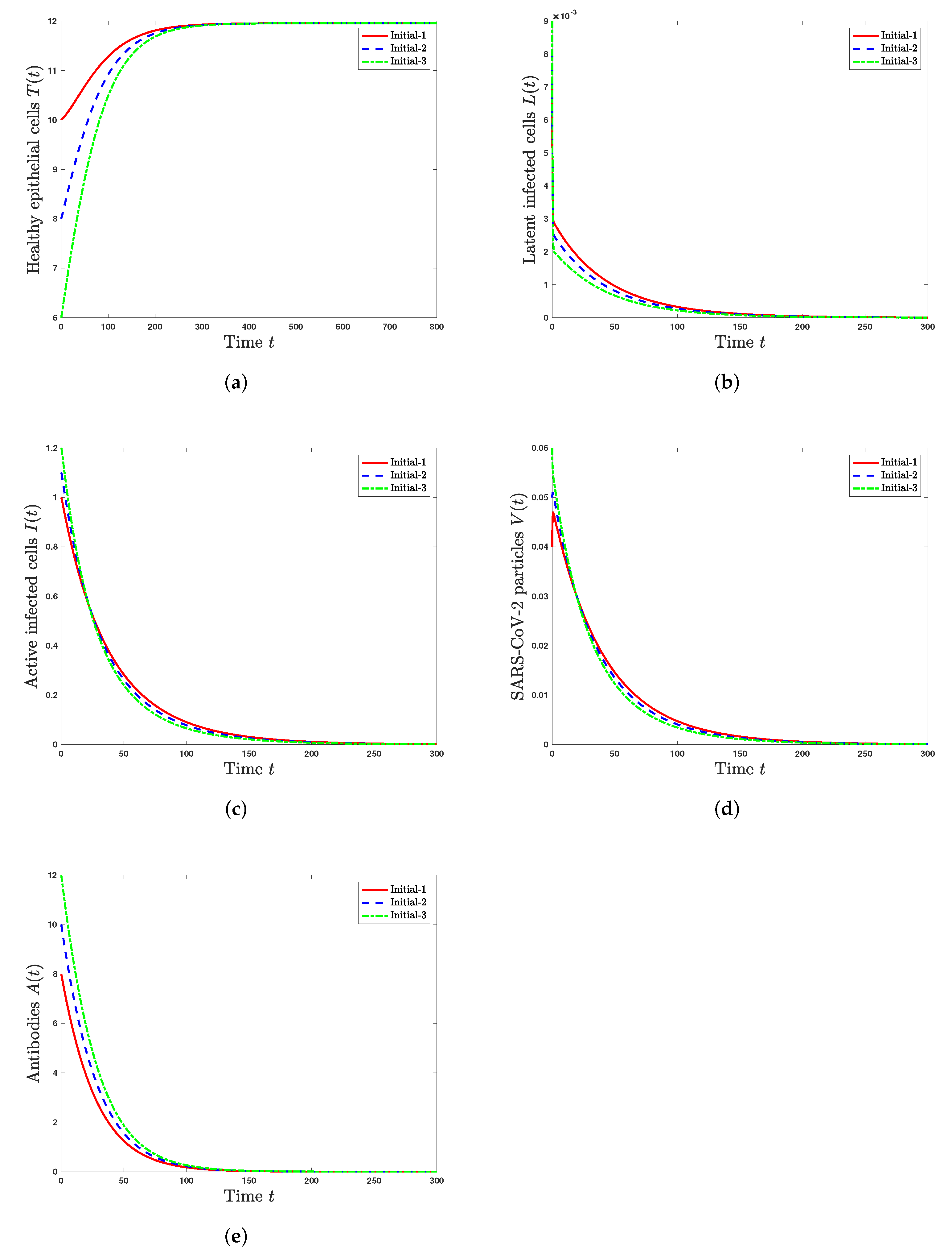
Scenario1 (Stability of): and . Using these values, we compute and . According to Theorem 2, is GAS and SARS-CoV-2 is predicted to be completely cleared from the body. From Figure 1, we see that the numerical results confirm the results of Theorem 2. We note that the concentration of healthy epithelial cells is increased and converges to its normal value , while the concentrations of latent infected cells, active infected cells, SARS-CoV-2 particles, and antibodies are decaying and tend toward zero. In this situation, the virus particles will be eliminated from the body.
Scenario 2 (Stability of): and . This gives , , and . According to Theorem 3, is GAS. From Figure 2, we can see that there is agreement between the numerical and theoretical results of Theorem 3. In addition, the solutions of the system converge to the steady state . In such a case, SARS-CoV-2 exists but with an inactive antibody immune response.
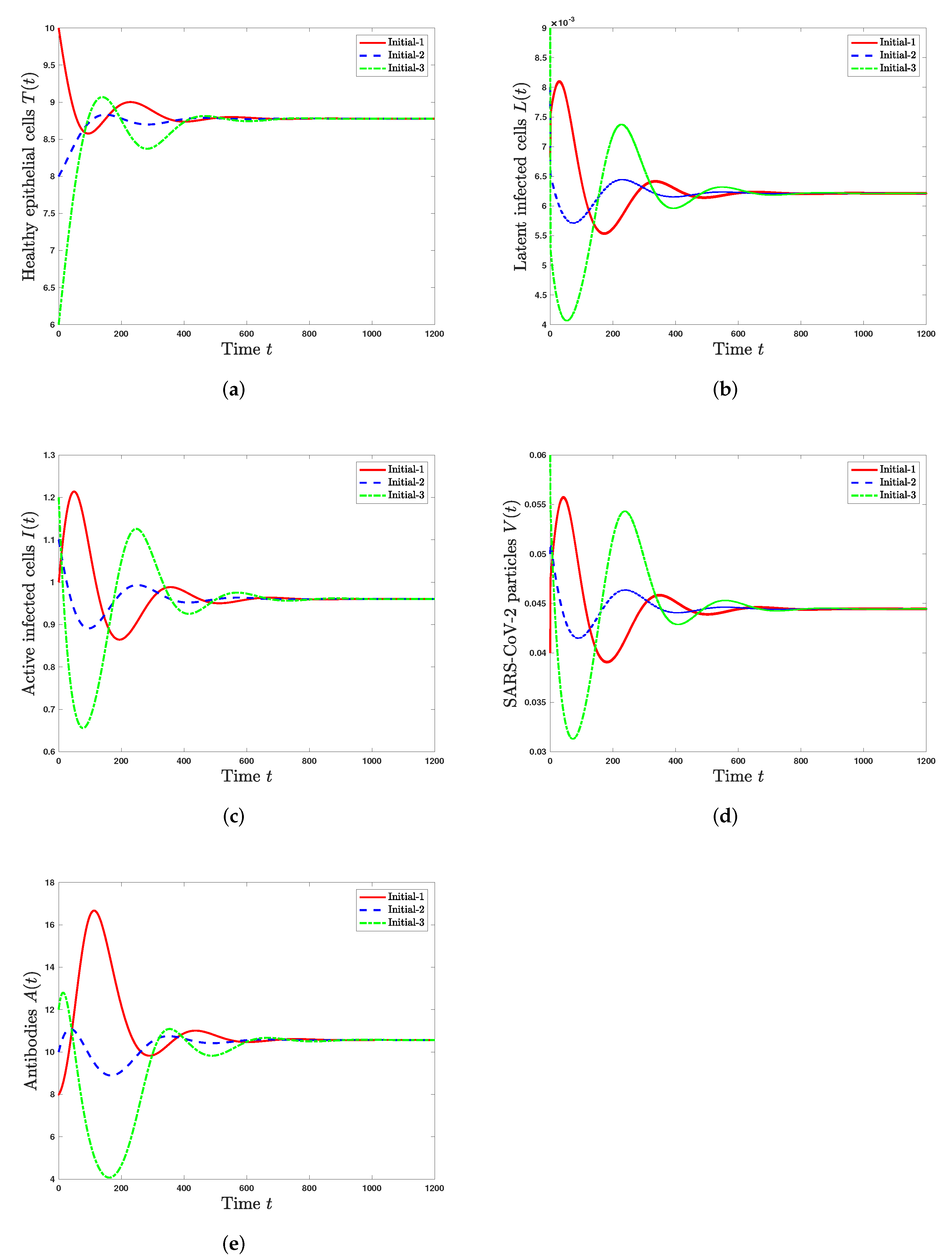
Scenario 3 (Stability of): and . These values give , , and . According to Theorem 4, is GAS. Further, the solutions of the system converge to the steady state . In this situation, SARS-CoV-2 exists with active antibody immunity (Figure 3).
5.2. Effect of the Time Delay on the SARS-CoV-2 Dynamics
In this subsection, we explore the impact of time delays on the stability of the steady states. We note from Equations (24) and (25) that the parameters and rely on the delay parameter , which causes a significant change in the stability of the system. To clarify this situation, we choose , , and is varied. Moreover, we consider the initial state initial-3. Figure 4 shows the influence of the time delay on the solution of the system. We notice that as time delay is increased, the number of healthy epithelial cells is increased, while the numbers of latent infected cells, active infected cells, SARS-CoV-2 particles, and antibodies are decreased. Now, let us write and as
We see that and are decreasing functions of . Let and be such that and . Using the values of the parameters, we obtain and . Therefore, we have the following cases:
(i) if , then and is GAS;
(ii) if , then and and is GAS;
(iii) if ,then and and is GAS. We can see from the above argumentation that increasing time delay values can have the same impact as antiviral treatment.
6. Conclusions and Discussion
In this paper, we formulate a COVID-19 infection model with distributed and discrete delays and an antibody immune response. Four time delays are included in the model: a delay in the formation of latent infected cells, a delay in the formation of active infected cells, a delay in the activation of latent infected cells, a maturation delay of new SARS-CoV-2 particles. We consider a logistic term for the healthy epithelial cells. We prove the nonnegativity and boundedness of the solutions. We calculate all steady states and establish that their existence is governed by two threshold parameters: the basic reproduction number and the antibody immune response activation number . The global stability of all steady states of the model is investigated by constructing Lyapunov functions and LaSalle’s invariance principal. We prove the following:
- The healthy steady state always exists and it is GAS when . This leads to the situation of an individual without SARS-CoV-2 infection.
- The infected steady state with an inactive antibody immune response exists if and . It is GAS when and . This represents the situation of SARS-CoV-2 infection in a patient with an inactive immune response.
- The infected steady state with active antibody immune response exists and it is GAS when and . This leads to the situation of SARS-CoV-2 infection in a patient with an active immune response.
We performed numerical simulations for the model and found that both the numerical and theoretical results are consistent. We studied the effect of time delays on the global dynamical properties of the model. We note that is a decreasing function on time delays , , , and . When all other parameters are fixed and delays are sufficiently large, becomes less than one, which makes the healthy steady state globally asymptotically stable. From a biological viewpoint, time delays play positive roles in the SARS-CoV-2 infection process in order to eliminate the virus. Sufficiently large time delays slow down SARS-CoV-2’s development, and SARS-CoV-2 is controlled and disappears. This offers some suggestions on new drugs to prolong the time for the formation of latent infected epithelial cells, the time for the formation of active infected epithelial cells, the time for the activation of latent infected epithelial cells, or the time for SARS-CoV-2 particles to mature (infectious).
The model investigated in this work can be developed by (i) using real data to estimate the parameters’ values and examine the validity of the model, (ii) considering the diffusion of SARS-CoV-2 particles and cells [61,62], (iii) expanding it to a multiscale model to obtain a deeper understanding of the SARS-CoV-2 dynamics [63,64], (iv) incorporating the role of CTLs in killing the active infected cells. If we consider system (1)–(5) under the effect of CTL immunity, system (1)–(5) is extended to the following model:
where represents the concentration of CTLs at time t. The active infected cells are killed by CTLs at rate . The terms and refer to the proliferation and death rates of CTLs, respectively. Studying the SARS-CoV-2 dynamics model with such extensions is left to future work.
Author Contributions
Conceptualization, A.M.E. and A.D.A.A.; Formal analysis, A.M.E., A.D.A.A. and A.D.H.; Investigation, A.J.A.; Methodology, A.M.E. and A.D.H.; Writing—original draft, A.J.A.; Writing—review & editing, A.D.A.A. All authors have read and agreed to the published version of the manuscript.
Funding
This project was funded by the Deanship of Scientific Research (DSR), King Abdulaziz University, Jeddah, Saudi Arabia, under grant no. (KEP-PHD-95-130-42).
Institutional Review Board Statement
Not applicable.
Informed Consent Statement
Not applicable.
Data Availability Statement
Not applicable.
Acknowledgments
This project was funded by the Deanship of Scientific Research (DSR), King Abdulaziz University, Jeddah, Saudi Arabia under grant no. (KEP-PHD-95-130-42). The authors, therefore, acknowledge with thanks DSR technical and financial support.
Conflicts of Interest
The authors declare no conflict of interest.
Appendix A
MATLAB scripts
function H = COVID (t,y,Z)
global lambda beta eta tau1 tau2 tau3 tau4 alpha d1 d2 d3 d4 d5 r k u q n1 n2 n3 n4 Tmax
ylag1 = Z (:,1); ylag2 = Z (:,2); ylag3 = Z (:,3); ylag4 = Z (:,4);
H=zeros (5,1);
H (1)=lambda-d1*y (1)+r*y (1)*(1-y (1)/Tmax)-beta*y (1)*y (4);
H (2)=eta*beta*exp (-n1*tau1)*ylag1 (1)*ylag1 (4)-(alpha+d2)*y (2);
H (3)=(1-eta)*beta*exp (-n2*tau2)*ylag2 (1)*ylag2 (4)+alpha*exp (-n3*tau3)*ylag3 (2)-d3*y (3);
H (4)=k*exp (-n4*tau4)*ylag4 (3)-d4*y (4)-u*y (4)*y (5);
H (5)=q*y (4)*y (5)-d5*y (5);
end
Main Programm
global lambda beta eta tau1 tau2 tau3 tau4 alpha d1 d2 d3 d4 d5 r k u q n1 n2 n3 n4 Tmax
caseNumber=3;
j=1;
if caseNumber==1
beta=0.05;
q=0.1;
end
if caseNumber==2
beta=0.13;
q=0.1;
end
if caseNumber==3
beta=0.13;
q=0.9;
end
%===== Fixed data =======
lambda=0.11; r=0.01; Tmax=13; eta=0.5; alpha=4.08; k=0.25; u=0.05; d1=0.01; d2=1e-3; d3=0.05; d4=4.36; d5=0.04; n1=0.001; n2=0.11; n3=1; n4=1;
%==== Delay parameters =====
tau1=0.1; tau2=0.1; tau3=0.1; tau4=0.1;
%===Initial conditions =====
a0=10;b0=0.007;c0=1.;d0=0.04;e0=8;
sol12 = dde23 (’COVID’,[tau1 tau2 tau3 tau4],[a0; b0; c0; d0; e0], [0 1200]);
figure (1)
pp0=plot (sol12.x, sol12.y(j,:));
References
- World Health Organization (WHO). Coronavirus Disease (COVID-19), Weekly Epidemiological Update. 2022. Available online: https://www.who.int/emergencies/diseases/novel-coronavirus-2019/situation-reports (accessed on 16 January 2022).
- Huang, C.; Wang, Y.; Li, X.; Ren, L.; Zhao, J.; Hu, Y.; Zhang, L.; Fan, G.; Xu, J.; Gu, X.; et al. Clinical features of patients infected with 2019 novel coronavirus in wuhan, china. Lancet 2020, 395, 497–506. [Google Scholar] [CrossRef] [Green Version]
- Abuin, P.; Anderson, A.; Ferramosca, A.; Hernandez-Vargas, E.A.; Gonzalez, A.H. Characterization of SARS-CoV-2 dynamics in the host. Annu. Rev. Control 2020, 50, 457–468. [Google Scholar] [CrossRef] [PubMed]
- World Health Organization (WHO). Coronavirus Disease (COVID-19). Vaccine Tracker. 2021. Available online: https://covid19.trackvaccines.org/agency/who/ (accessed on 1 April 2022).
- Varga, Z.; Flammer, A.J.; Steiger, P.; Haberecker, M.; Andermatt, R.; Zinkernagel, A.S. Endothelial cell infection and endotheliitis in COVID-19. Lancet 2020, 395, 1417–1418. [Google Scholar] [CrossRef]
- Du, S.Q.; Yuan, W. Mathematical modeling of interaction between innate and adaptive immune responses in COVID-19 and implications for viral pathogenesis. J. Med. Virol. 2020, 92, 1615–1628. [Google Scholar] [CrossRef]
- Currie, C.; Fowler, J.; Kotiadis, K.; Monks, T. How simulation modelling can help reduce the impact of COVID-19. J. Simul. 2020, 14, 83–97. [Google Scholar] [CrossRef] [Green Version]
- Fredj, H.B.; Chérif, F. Novel corona virus disease infection in Tunisia: Mathematical model and the impact of the quarantine strategy. Chaos Solitons Fractals 2020, 138, 109969. [Google Scholar] [CrossRef]
- Browne, C.J.; Gulbudak, H.; Macdonald, J.C. Differential impacts of contact tracing and lockdowns on outbreak size in COVID-19 model applied to China. J. Theor. Biol. 2022, 532, 110919. [Google Scholar] [CrossRef]
- Anderson, R.M.; Heesterbeek, H.; Klinkenberg, D.; Hollingsworth, T.D. How will country-based mitigation measures influence the course of the COVID-19 epidemic? Lancet 2020, 395, 931–934. [Google Scholar] [CrossRef]
- Davies, N.G.D.; Kucharski, A.J.; Eggo, R.M.; Gimma, A.; Edmunds, W.J.; Jombart, T. Effects of non-pharmaceutical interventions on COVID-19 cases, deaths, and demand for hospital services in the UK: A modelling study. Lancet Public Health 2020, 5, 375–385. [Google Scholar] [CrossRef]
- Ferretti, L.; Wymant, C.; Kendall, M.; Zhao, L.; Nurtay, A.; Abeler-Dorner, L.; Parker, M.; Bonsall, D.; Fraser, C. Quantifying SARS-CoV-2 transmission suggests epidemic control with digital contact tracing. Science 2020, 368, eabb6936. [Google Scholar] [CrossRef] [Green Version]
- Krishna, M.V.; Prakash, J. Mathematical modelling on phase based transmissibility of coronavirus. Infect. Dis. Model. 2020, 5, 375–385. [Google Scholar] [CrossRef] [PubMed]
- Ferguson, N.M.; Laydon, D.; Nedjati-Gilani, G.; Imai, N.; Ainslie, K.; Baguelin, M.; Bhatia, S.; Boonyasiri, A.; Cucunubá, Z.; Cuomo-Dannenburg, G.; et al. Impact of Non-Pharmaceutical Interventions (NPIs) to Reduce COVID-19 Mortality and Healthcare Demand; Technical Report; Imperial College London: London, UK, 2020. [Google Scholar]
- Bellomo, N.; Bingham, R.; Chaplain, M.A.J.; Dosi, G.; Forni, G.; Knopoff, D.A.; Lowengrub, J.; Twarock, R.; Virgillito, M.E. A multiscale model of virus pandemic: Heterogeneous interactive entities in a globally connected world. Math. Model. Methods Appl. Sci. 2020, 30, 1591–1651. [Google Scholar] [CrossRef] [PubMed]
- Fatehi, F.; Bingham, R.J.; Dykeman, E.C.; Stockley, P.G.; Twarock, R. Comparing antiviral strategies against COVID-19 via multiscale within-host modelling. R. Soc. Open Sci. 2021, 8, 210082. [Google Scholar] [CrossRef]
- Perelson, A.S.; Ke, R. Mechanistic modeling of SARS-CoV-2 and other infectious diseases and the effects of therapeutics. Clin. Pharmacol. Ther. 2021, 109, 829–840. [Google Scholar] [CrossRef] [PubMed]
- Li, C.; Xu, J.; Liu, J.; Zhou, Y. The within-host viral kinetics of SARS-CoV-2. Math. Biosci. Eng. 2020, 17, 2853–2861. [Google Scholar] [CrossRef] [PubMed]
- Danchin, A.; Pagani-Azizi, O.; Turinici, G.; Yahiaoui, G. COVID-19 adaptive humoral immunity models: Non-neutralizing versus antibody-disease enhancement scenarios. medRxiv 2020. [Google Scholar]
- Sadria, M.; Layton, A.T. Modeling within-host SARS-CoV-2 infection dynamics and potential treatments. Viruses 2021, 13, 1141. [Google Scholar] [CrossRef]
- Néant, N.; Lingas, G.; Hingrat, Q.L.; Ghosn, J.; Engelmann, I.; Lepiller, Q.; Gaymard, A.; Ferrxex, V.; Hartard, C.; Plantier, J.-C.; et al. Modeling SARS-CoV-2 viral kinetics and association with mortality in hospitalized patients from the French COVID cohort. Proc. Natl. Acad. Sci. USA 2021, 118, e2017962118. [Google Scholar] [CrossRef]
- Pinky, L.; Dobrovolny, H.M. SARS-CoV-2 coinfections: Could influenza and the common cold be beneficial? J. Med. Virol. 2020, 92, 2623–2630. [Google Scholar] [CrossRef]
- Hernandez-Vargas, E.A.; Velasco-Hernandez, J.X. In-host mathematical modelling of COVID-19 in humans. Annu. Rev. Control. 2020, 50, 448–456. [Google Scholar] [CrossRef]
- Blanco-Rodríguez, R.; Du, X.; Hernández-Vargas, E.A. Computational simulations to dissect the cell immune response dynamics for severe and critical cases of SARS-CoV-2 infection. Comput. Methods Programs Biomed. 2021, 211, 106412. [Google Scholar] [CrossRef] [PubMed]
- Blanco-Rodríguez, R.; Du, X.; Hernández-Vargas, E.A. Untangling the cell immune response dynamic for severe and critical cases, of SARS-CoV-2 infection. bioRxiv 2020. [Google Scholar] [CrossRef]
- Ke, R.; Zitzmann, C.; Ho, D.D.; Ribeiro, R.M.; Perelson, A.S. In vivo kinetics of SARS-CoV-2 infection and its relationship with a person’s infectiousness. Proc. Natl. Acad. Sci. USA 2021, 118, e2111477118. [Google Scholar] [CrossRef] [PubMed]
- Ghosh, I. Within host dynamics of SARS-CoV-2 in humans: Modeling immune responses and antiviral treatments. SN Comput. Sci. 2021, 2, 482. [Google Scholar] [CrossRef] [PubMed]
- Wang, S.; Pan, Y.; Wang, Q.; Miao, H.; Brown, A.N.; Rong, L. Modeling the viral dynamics of SARS-CoV-2 infection. Math. Biosci. 2020, 1328, 08438. [Google Scholar] [CrossRef]
- Almoceraa, A.E.S.; Quiroz, G.; Hernandez-Vargas, E.A. Stability analysis in COVID-19 within-host model with immune response. Commun. Nonlinear Sci. Numer. Simul. 2021, 95, 105584. [Google Scholar] [CrossRef]
- Hattaf, K.; Yousfi, N. Dynamics of SARS-CoV-2 infection model with two modes of transmission and immune response. Math. Biosci. Eng. 2020, 17, 5326–5340. [Google Scholar] [CrossRef]
- Chatterjee, A.N.; Basir, F.A. A model for SARS-CoV-2 infection with treatment. Comput. Math. Methods Med. 2020, 2020, 1352982. [Google Scholar] [CrossRef]
- Mondal, J.; Samui, P.; Chatterjee, A.N. Dynamical demeanour of SARS-CoV-2 virus undergoing immune response mechanism in COVID-19 pandemic. Eur. Phys. J. Spec. Top. 2022. [Google Scholar] [CrossRef]
- Nath, B.J.; Dehingia, K.; Mishra, V.N.; Chu, Y.-M.; Sarmah, H.K. Mathematical analysis of a within-host model of SARS-CoV-2. Adv. Differ. Equ. 2021, 2021, 113. [Google Scholar] [CrossRef]
- Ghanbari, B. On fractional approaches to the dynamics of a SARS-CoV-2 infection model including singular and non-singular kernels. Results Phys. 2021, 28, 104600. [Google Scholar] [CrossRef] [PubMed]
- Khan, H.; Ahmad, F.; Tunç, O.; Idrees, M. On fractal-fractional Covid-19 mathematical model. Chaos Solitons Fractals 2022, 157, 111937. [Google Scholar] [CrossRef]
- Pandey, P.; Gómez-Aguilar, J.F.; Kaabar, M.K.; Siri, Z.; Allah, A.M.A. Mathematical modeling of COVID-19 pandemic in India using Caputo-Fabrizio fractional derivative. Comput. Biol. Med. 2022, 145, 105518. [Google Scholar] [CrossRef] [PubMed]
- Elaiw, A.M.; Hobiny, A.D.; Agha, A.D.A. Global dynamics of SARS-CoV-2/cancer model with immune responses. Appl. Math. Comput. 2021, 408, 126364. [Google Scholar] [CrossRef] [PubMed]
- Elaiw, A.M.; Agha, A.D.A.; Azoz, S.A.; Ramadan, E. Global analysis of within-host SARS-CoV-2/HIV coinfection model with latency. Eur. Phys. J. Plus 2022, 137, 174. [Google Scholar] [CrossRef] [PubMed]
- Agha, A.D.A.; Elaiw, A.M. Global dynamics of SARS-CoV-2/malaria model with antibody immune response. Math. Biosci. Eng. 2022. accepted. [Google Scholar]
- Perkins, T.A.; España, G. Optimal control of the COVID-19 pandemic with non-pharmaceutical interventions. Bull. Math. Biol. 2020, 82, 1–24. [Google Scholar] [CrossRef]
- Balcha, S.F.; Obsu, L.L. Optimal control strategies for the transmission risk of COVID-19. J. Biol. Dyn. 2020, 14, 590–607. [Google Scholar]
- Libotte, G.B.; Lobato, F.S.; Platt, G.M.; Neto, A.J.S. Determination of an optimal control strategy for vaccine administration in COVID-19 pandemic treatment. Comput. Methods Programs Biomed. 2020, 196, 105664. [Google Scholar] [CrossRef]
- Shen, Z.H.; Chu, Y.M.; Khan, M.A.; Muhammad, S.; Al-Hartomy, O.A.; Higazy, M. Mathematical modeling and optimal control of the COVID-19 dynamics. Results Phys. 2021, 31, 105028. [Google Scholar] [CrossRef]
- Asamoah, J.K.K.; Okyere, E.; Abidemi, A.; Moore, S.E.; Sun, G.Q.; Jin, Z.; Acheampong, E.; Gordon, J.F. Optimal control and comprehensive cost-effectiveness analysis for COVID-19. Results Phys. 2022, 33, 105177. [Google Scholar] [CrossRef] [PubMed]
- Kirschner, D.; Lenhart, S.; Serbin, S. Optimal control of the chemotherapy of HIV. J. Math. Biol. 1997, 35, 775–792. [Google Scholar] [CrossRef] [PubMed] [Green Version]
- Elaiw, A.M.; Xia, X. HIV dynamics: Analysis and robust multirate MPC-based treatment schedules. J. Math. Anal. Appl. 2009, 359, 285–301. [Google Scholar] [CrossRef] [Green Version]
- Alrabaiah, H.; Safi, M.A.; DarAssi, M.H.; Al-Hdaibat, B.; Ullah, S.; Khan, M.A.; Shah, S.A.A. Optimal control analysis of hepatitis B virus with treatment and vaccination. Results Phys. 2020, 19, 103599. [Google Scholar] [CrossRef]
- Mojaver, A.; Kheiri, H. Dynamical analysis of a class of hepatitis C virus infection models with application of optimal control. Int. J. Biomath. 2016, 9, 1650038. [Google Scholar] [CrossRef]
- Nowak, M.A.; Bangham, C.R.M. Population dynamics of immune responses to persistent viruses. Science 1996, 272, 74–79. [Google Scholar] [CrossRef] [Green Version]
- Chhetri, B.; Bhagat, V.M.; Vamsi, D.K.K.; Ananth, V.S.; Prakash, D.B.; Mandale, R.; Muthusamy, S.; Sanjeevi, C.B. Within-host mathematical modeling on crucial inflammatory mediators and drug interventions in COVID-19 identifies combination therapy to be most effective and optimal. Alex. Eng. J. 2021, 60, 2491–2512. [Google Scholar] [CrossRef]
- Chatterjee, A.N.; Basir, F.A.; Almuqrin, M.A.; Mondal, J.; Khan, I. SARS-CoV-2 infection with lytic and nonlytic immune responses: A fractional order optimal control theoretical study. Results Phys. 2021, 26, 104260. [Google Scholar] [CrossRef]
- Fadai, N.T.; Sachak-Patwa, R.; Byrne, H.M.; Maini, P.K.; Bafadhel, M.; Nicolau, D.V., Jr. Infection, inflammation and intervention: Mechanistic modelling of epithelial cells in COVID-19. J. R. Soc. Interface 2021, 18, 20200950. [Google Scholar] [CrossRef]
- Bar-On, Y.M.; Flamholz, A.; Phillips, R.; Milo, R. Science Forum: SARS-CoV-2 (COVID-19) by the numbers. elife 2020, 9, e57309. [Google Scholar] [CrossRef]
- Zhou, X.; Zhang, L.; Zheng, T.; Li, H.; Teng, Z. Global stability for a delayed HIV reactivation model with latent infection and Beddington-DeAngelis incidence. Appl. Math. Lett. 2021, 117, 1–10. [Google Scholar] [CrossRef]
- Hale, J.K.; Lunel, S.M.V. Introduction to Functional Differential Equations; Springer: New York, NY, USA, 1993. [Google Scholar]
- Yang, X.; Chen, S.; Chen, J. Permanence and positive periodic solution for the single-species nonautonomous delay diffusive models. Comput. Math. Appl. 1996, 32, 109–116. [Google Scholar] [CrossRef] [Green Version]
- Driessche, P.V.; Watmough, J. Reproduction numbers and sub-threshold endemic equilibria for compartmental models of disease transmission. Math. Biosci. 2002, 180, 29–48. [Google Scholar] [CrossRef]
- Ciupe, S.M.; Heffernan, J.M. In-host modeling. Infect. Dis. Model. 2017, 2, 188–202. [Google Scholar] [CrossRef] [PubMed]
- Korobeinikov, A. Global properties of basic virus dynamics models. Bull. Math. Biol. 2004, 66, 879–883. [Google Scholar] [CrossRef]
- LaSalle, J.P. The Stability of Dynamical Systems; SIAM: Philadelphia, PA, USA, 1976. [Google Scholar]
- Bellomo, N.; Tao, Y. Stabilization in a chemotaxis model for virus infection. Discret. Contin. Dyn. Syst. Ser. S 2020, 13, 105–117. [Google Scholar] [CrossRef] [Green Version]
- Elaiw, A.M.; Agha, A.D.A.; Alshaikh, M.A. Global stability of a within-host SARS-CoV-2/cancer model with immunity and diffusion. Int. J. Biomath. 2021, 15, 2150093. [Google Scholar] [CrossRef]
- Bellomo, N.; Burini, D.; Outada, N. Multiscale models of Covid-19 with mutations and variants. Netw. Heterog. Media 2022, 17, 293–310. [Google Scholar] [CrossRef]
- Bellomo, N.; Burini, D.; Outada, N. Pandemics of mutating virus and society: A multi-scale active particles approach. Philos. Trans. Ser. A Math. Phys. Eng. Sci. 2022, 380, 1–14. [Google Scholar] [CrossRef]
Figure 1.
Solutions of system (19)–(23) with three initial conditions when . (a) Healthy epithelial cells; (b) latent infected cells; (c) active infected cells; (d) SARS-CoV-2 particles; (e) antibodies.
Figure 1.
Solutions of system (19)–(23) with three initial conditions when . (a) Healthy epithelial cells; (b) latent infected cells; (c) active infected cells; (d) SARS-CoV-2 particles; (e) antibodies.

Figure 2.
Solutions of system (19)–(23) with three initial conditions when and . (a) Healthy epithelial cells; (b) latent infected cells; (c) active infected cells; (d) SARS-CoV-2 particles; (e) antibodies.
Figure 2.
Solutions of system (19)–(23) with three initial conditions when and . (a) Healthy epithelial cells; (b) latent infected cells; (c) active infected cells; (d) SARS-CoV-2 particles; (e) antibodies.

Figure 3.
Solutions of system (19)–(23) with three initial conditions when and . (a) Healthy epithelial cells; (b) latent infected cells; (c) active infected cells; (d) SARS-CoV-2 particles; (e) antibodies.
Figure 3.
Solutions of system (19)–(23) with three initial conditions when and . (a) Healthy epithelial cells; (b) latent infected cells; (c) active infected cells; (d) SARS-CoV-2 particles; (e) antibodies.

Figure 4.
Solutions of system (19)–(23) under the influence of the time delay . (a) Healthy epithelial cells; (b) latent infected cells; (c) active infected cells; (d) SARS-CoV-2 particles; (e) antibodies.
Figure 4.
Solutions of system (19)–(23) under the influence of the time delay . (a) Healthy epithelial cells; (b) latent infected cells; (c) active infected cells; (d) SARS-CoV-2 particles; (e) antibodies.

Publisher’s Note: MDPI stays neutral with regard to jurisdictional claims in published maps and institutional affiliations. |
© 2022 by the authors. Licensee MDPI, Basel, Switzerland. This article is an open access article distributed under the terms and conditions of the Creative Commons Attribution (CC BY) license (https://creativecommons.org/licenses/by/4.0/).
Share and Cite
MDPI and ACS Style
Elaiw, A.M.; Alsaedi, A.J.; Al Agha, A.D.; Hobiny, A.D. Global Stability of a Humoral Immunity COVID-19 Model with Logistic Growth and Delays. Mathematics 2022, 10, 1857. https://doi.org/10.3390/math10111857
AMA Style
Elaiw AM, Alsaedi AJ, Al Agha AD, Hobiny AD. Global Stability of a Humoral Immunity COVID-19 Model with Logistic Growth and Delays. Mathematics. 2022; 10(11):1857. https://doi.org/10.3390/math10111857
Chicago/Turabian StyleElaiw, Ahmed M., Abdullah J. Alsaedi, Afnan Diyab Al Agha, and Aatef D. Hobiny. 2022. "Global Stability of a Humoral Immunity COVID-19 Model with Logistic Growth and Delays" Mathematics 10, no. 11: 1857. https://doi.org/10.3390/math10111857
Note that from the first issue of 2016, this journal uses article numbers instead of page numbers. See further details here.