
How Seasonality and Control Measures Jointly Determine the Multistage Waves of the COVID-19 Epidemic: A Modelling Study and Implications


Abstract
:1. Introduction
2. Materials and Methods
3. Results
4. Discussion
5. Conclusions
Author Contributions
Funding
Institutional Review Board Statement
Informed Consent Statement
Data Availability Statement
Conflicts of Interest
References
- Fukutome, A.; Watashi, K.; Kawakami, N.; Ishikawa, H. Mathematical modeling of severe acute respiratory syndrome nosocomial transmission in Japan: The dynamics of incident cases and prevalent cases. Microbiol. Immunol. 2007, 51, 823–832. [Google Scholar] [CrossRef] [Green Version]
- Oraby, T.; Tyshenko, M.G.; Balkhy, H.H.; Tasnif, Y.; Quiroz-Gaspar, A.; Mohamed, Z.; Araya, A.; Elsaadany, S.; Al-Mazroa, E.; Alhelail, M.A.; et al. Analysis of the Healthcare MERS-CoV Outbreak in King Abdulaziz Medical Center, Riyadh, Saudi Arabia, June-August 2015 Using a SEIR Ward Transmission Model. Int. J. Environ. Res. Public Health 2020, 17, 2936. [Google Scholar] [CrossRef]
- Khedher, N.B.; Kolsi, L.; Alsaif, H. A multi-stage SEIR model to predict the potential of a new COVID-19 wave in KSA after lifting all travel restrictions. Alex. Eng. J. 2021, 60, 3965–3974. [Google Scholar] [CrossRef]
- COVID-19 Coronavirus Pandemic. Available online: https://www.worldometers.info/coronavirus (accessed on 20 March 2022).
- Lopez, L.; Rodo, X. A modified SEIR model to predict the COVID-19 outbreak in Spain and Italy: Simulating control scenarios and multi-scale epidemics. Results Phys. 2021, 21, 103746. [Google Scholar] [CrossRef]
- Liu, X.; Huang, J.; Li, C.; Zhao, Y.; Wang, D.; Huang, Z.; Yang, K. The role of seasonality in the spread of COVID-19 pandemic. Environ. Res. 2021, 195, 110874. [Google Scholar] [CrossRef]
- Wang, H.; Xu, K.; Li, Z.; Pang, K.; He, H. Improved Epidemic Dynamics Model and Its Prediction for COVID-19 in Italy. Appl. Sci. 2020, 10, 4930. [Google Scholar] [CrossRef]
- Zhang, R.; Li, Y.; Zhang, A.; Wang, Y.; Molina, M.J. Identifying airborne transmission as the dominant route for the spread of COVID-19. Proc. Natl. Acad. Sci. USA 2020, 117, 14857–14863. [Google Scholar] [CrossRef]
- Ruan, L.; Wen, M.; Zeng, Q.; Chen, C.; Huang, S.; Yang, S.; Yang, J.; Wang, J.; Hu, Y.; Ding, S.; et al. New Measures for the Coronavirus Disease 2019 Response: A Lesson from the Wenzhou Experience. Clin. Infect. Dis. 2020, 71, 866–869. [Google Scholar] [CrossRef] [Green Version]
- Nistal, R.; de la Sen, M.; Gabirondo, J.; Alonso-Quesada, S.; Garrido, A.J.; Garrido, I. A Study on COVID-19 Incidence in Europe through Two SEIR Epidemic Models Which Consider Mixed Contagions from Asymptomatic and Symptomatic Individuals. Appl. Sci. 2021, 14, 6266. [Google Scholar] [CrossRef]
- Hellewell, J.; Abbott, S.; Gimma, A.; Bosse, N.I.; Jarvis, C.I.; Russell, T.W.; Munday, J.D.; Kucharski, A.J.; Edmunds, W.J.; Sun, F.; et al. Feasibility of controlling COVID-19 outbreaks by isolation of cases and contacts. Lancet Glob. Health 2020, 8, e488–e496. [Google Scholar] [CrossRef] [Green Version]
- Pan, A.; Liu, L.; Wang, C.; Guo, H.; Hao, X.; Wang, Q.; Huang, J.; He, N.; Yu, H.; Lin, X.; et al. Association of Public Health Interventions with the Epidemiology of the COVID-19 Outbreak in Wuhan, China. JAMA 2020, 323, 1915–1923. [Google Scholar] [CrossRef] [Green Version]
- Prem, K.; Liu, Y.; Russell, T.W.; Kucharski, A.J.; Eggo, R.M.; Davies, N.; Flasche, S.; Clifford, S.; Pearson, C.A.; Munday, J.D.; et al. The effect of control strategies to reduce social mixing on outcomes of the COVID-19 epidemic in Wuhan, China: A modelling study. Lancet Public Health 2020, 5, e261–e270. [Google Scholar] [CrossRef] [Green Version]
- Batabyal, S. COVID-19: Perturbation dynamics resulting chaos to stable with seasonality transmission. Chaos Solitons Fractals 2021, 145, 110772. [Google Scholar] [CrossRef]
- Neher, R.A.; Dyrdak, R.; Druelle, V.; Hodcroft, E.B.; Albert, J. Potential impact of seasonal forcing on a SARS-CoV-2 pandemic. Swiss Med. Wkly. 2020, 150, w20224. [Google Scholar] [CrossRef] [Green Version]
- Steel, J.; Palese, P.; Lowen, A.C. Transmission of a 2009 pandemic influenza virus shows a sensitivity to temperature and humidity similar to that of an H3N2 seasonal strain. J. Virol. 2011, 85, 1400–1402. [Google Scholar] [CrossRef] [Green Version]
- Eccles, R. An explanation for the seasonality of acute upper respiratory tract viral infections. Acta Otolaryngol. 2002, 122, 183–191. [Google Scholar] [CrossRef]
- Huang, Z.; Huang, J.; Gu, Q.; Du, P.; Liang, H.; Dong, Q. Optimal temperature zone for the dispersal of COVID-19. Sci. Total Environ. 2020, 736, 139487. [Google Scholar] [CrossRef]
- Yao, M.; Zhang, L.; Ma, J.; Zhou, L. On airborne transmission and control of SARS-Cov-2. Sci. Total Environ. 2020, 731, 139178. [Google Scholar] [CrossRef]
- Coskun, H.; Yildirim, N.; Gunduz, S. The spread of COVID-19 virus through population density and wind in Turkey cities. Sci. Total Environ. 2021, 751, 141663. [Google Scholar] [CrossRef]
- Rendana, M. Impact of the wind conditions on COVID-19 pandemic: A new insight for direction of the spread of the virus. Urban Clim. 2020, 34, 100680. [Google Scholar] [CrossRef]
- Van Doremalen, N.; Bushmaker, T.; Morris, D.H.; Holbrook, M.G.; Gamble, A.; Williamson, B.N.; Tamin, A.; Harcourt, J.L.; Thornburg, N.J.; Gerber, S.I.; et al. Aerosol and Surface Stability of SARS-CoV-2 as Compared with SARS-CoV-1. N. Engl. J. Med. 2020, 382, 1564–1567. [Google Scholar] [CrossRef]
- Xie, J.; Zhu, Y. Association between ambient temperature and COVID-19 infection in 122 cities from China. Sci. Total Environ. 2020, 724, 138201. [Google Scholar] [CrossRef]
- Yao, Y.; Pan, J.; Liu, Z.; Meng, X.; Wang, W.; Kan, H.; Wang, W. No association of COVID-19 transmission with temperature or UV radiation in Chinese cities. Eur. Respir. J. 2020, 55. [Google Scholar] [CrossRef] [Green Version]
- Jüni, P.; Rothenbühler, M.; Bobos, P.; Thorpe, K.E.; Da Costa, B.R.; Fisman, D.N.; Slutsky, A.S.; Gesink, D. Impact of climate and public health interventions on the COVID-19 pandemic: A prospective cohort study. Can. Med. Assoc. J. 2020, 192, E566–E573. [Google Scholar] [CrossRef]
- Meyer, A.; Sadler, R.; Faverjon, C.; Cameron, A.R.; Bannister-Tyrrell, M. Evidence That Higher Temperatures Are Associated with a Marginally Lower Incidence of COVID-19 Cases. Front. Public Health 2020, 8, 367. [Google Scholar] [CrossRef]
- Lowen, A.C.; Steel, J.; Mubareka, S.; Palese, P. High temperature (30 degrees C) blocks aerosol but not contact transmission of influenza virus. J. Virol. 2008, 82, 5650–5652. [Google Scholar] [CrossRef] [Green Version]
- Kissler, S.M.; Tedijanto, C.; Goldstein, E.; Grad, Y.H.; Lipsitch, M. Projecting the transmission dynamics of SARS-CoV-2 through the postpandemic period. Science 2020, 368, 860–868. [Google Scholar] [CrossRef]
- Yarsky, P. Using a genetic algorithm to fit parameters of a COVID-19 SEIR model for US states. Math. Comput. Simul. 2021, 185, 687–695. [Google Scholar] [CrossRef]
- Bashir, M.F.; Benghoul, M.; Numan, U.; Shakoor, A.; Komal, B.; Bashir, M.A.; Bashir, M.; Tan, D. Environmental pollution and COVID-19 outbreak: Insights from Germany. Air Qual. Atmos. Health 2020, 13, 1385–1394. [Google Scholar] [CrossRef]
- Coccia, M. Factors determining the diffusion of COVID-19 and suggested strategy to prevent future accelerated viral infectivity similar to COVID. Sci. Total Environ. 2020, 729, 138474. [Google Scholar] [CrossRef]
- Mollalo, A.; Vahedi, B.; Rivera, K.M. GIS-based spatial modeling of COVID-19 incidence rate in the continental United States. Sci. Total Environ. 2020, 728, 138884. [Google Scholar] [CrossRef] [PubMed]
- Lian, X.; Huang, J.; Zhang, L.; Liu, C.; Liu, X.; Wang, L. Environmental Indicator for COVID-19 Non-Pharmaceutical Interventions. Geophys. Res. Lett. 2021, 149, 2020GL090344. [Google Scholar] [CrossRef] [PubMed]
- Li, W.; Gong, J.; Zhou, J.; Zhang, L.; Wang, D.; Li, J.; Shi, C.; Fan, H. An evaluation of COVID-19 transmission control in Wenzhou using a modified SEIR model. Epidemiol. Infect. 2021, 149, e2. [Google Scholar] [CrossRef] [PubMed]
- Carcione, J.M.; Santos, J.E.; Bagaini, C.; Ba, J. A Simulation of a COVID-19 Epidemic Based on a Deterministic SEIR Model. Front. Public Health 2020, 8, 230. [Google Scholar] [CrossRef] [PubMed]
- Chowell, G.; Hengartner, N.W.; Castillo-Chavez, C.; Fenimore, P.W.; Hyman, J.M. The basic reproductive number of Ebola and the effects of public health measures: The cases of Congo and Uganda. J. Theor. Biol. 2004, 229, 119–126. [Google Scholar] [CrossRef] [PubMed] [Green Version]
- Sun, D.; Long, X.; Liu, J. Modeling the COVID-19 Epidemic with Multi-Population and Control Strategies in the United States. Front. Public Health 2021, 9, 751940. [Google Scholar] [CrossRef]
- Liu, Z.; Magal, P.; Seydi, O.; Webb, G. Understanding Unreported Cases in the COVID-19 Epidemic Outbreak in Wuhan, China, and the Importance of Major Public Health Interventions. Biology 2020, 9, 50. [Google Scholar] [CrossRef] [Green Version]
- Yadav, P.D.; Sapkal, G.N.; Ella, R.; Sahay, R.R.; Nyayanit, D.A.; Patil, D.Y.; Deshpande, G.; Shete, A.M.; Gupta, N.; Mohan, V.K.; et al. Neutralization of Beta and Delta variant with sera of COVID-19 recovered cases and vaccinees of inactivated COVID-19 vaccine BBV152/Covaxin. J. Travel Med. 2021, 28, taab104. [Google Scholar] [CrossRef]
- Tareq, A.M.; Emran, T.B.; Dhama, K.; Dhawan, M.; Tallei, T.E. Impact of SARS-CoV-2 delta variant (B.1.617.2) in surging second wave of COVID-19 and efficacy of vaccines in tackling the ongoing pandemic. Hum. Vaccines Immunother. 2021, 17, 4126–4127. [Google Scholar] [CrossRef]
- Zhao, H.; Lu, L.; Peng, Z.; Chen, L.L.; Meng, X.; Zhang, C.; Ip, J.D.; Chan, W.M.; Chu, A.W.; Chan, K.H.; et al. SARS-CoV-2 Omicron variant shows less efficient replication and fusion activity when compared with delta variant in TMPRSS2-expressed cells. Emerg. Microbes Infect. 2022, 11, 277–283. [Google Scholar] [CrossRef]


| Countries | Outbreak Period 1 | Containment Period 1 | Outbreak Period 2 | Containment Period 2 | Outbreak Period 3 | Containment Period 3 |
|---|---|---|---|---|---|---|
| United States | 21 March 2020 | 1 May 2020 | NA | NA | 7 February 2021 | NA |
| France | 16 March 2020 | 11 May 2020 | 3 October 2020 | 11 November 2020 | 3 April 2020 | NA |
| Brazil | 25 March 2020 | 1 June 2020 | 24 November 2020 | NA | NA | NA |
| United Kingdom | 23 March 2020 | 11 May 2020 | 5 November 2020 | 2 December 2020 | 4 January 2021 | 17 May 2021 |
| Italy | 9 March 2020 | 4 May 2020 | 25 October 2020 | 10 January 2021 | 3 April 2021 | 2 June 2021 |
| Germany | 16 March 2020 | 20 April 2020 | 12 December 2020 | NA | NA | NA |
| Turkey | 1 April 2020 | 12 May 2020 | 8 November 2020 | 25 January 2021 | 29 April 2021 | 17 May 2021 |
| Australia | 2 March 2020 | 27 April 2020 | 2 August 2020 | 13 September 2020 | 1 January 2021 | 29 January 2021 |
| Spain | 13 March 2020 | 13 April 2020 | 25 October 2020 | 23 November 2020 | 8 January 2021 | 9 May 2021 |
| Argentina | 20 March 2020 | 16 May 2020 | 1 July 2020 | 18 July 2020 | 26 October 2020 | 1 December 2020 |
| South-Africa | 26 March 2020 | 1 June 2020 | 12 July 2020 | 17 August 2020 | 29 December 2020 | NA |
| Chile | 18 March 2020 | 7 August 2020 | 3 January 2021 | 23 March 2021 | NA | NA |
| Parameters | Upper and Lower Bounds |
|---|---|
| (0, 0.5] | |
| [0.1, 0.9] | |
| [1, 365] | |
| [0.1, 0.9] | |
| [0.8, 2.0] | |
| (0, 3] | |
| (0, 3] |
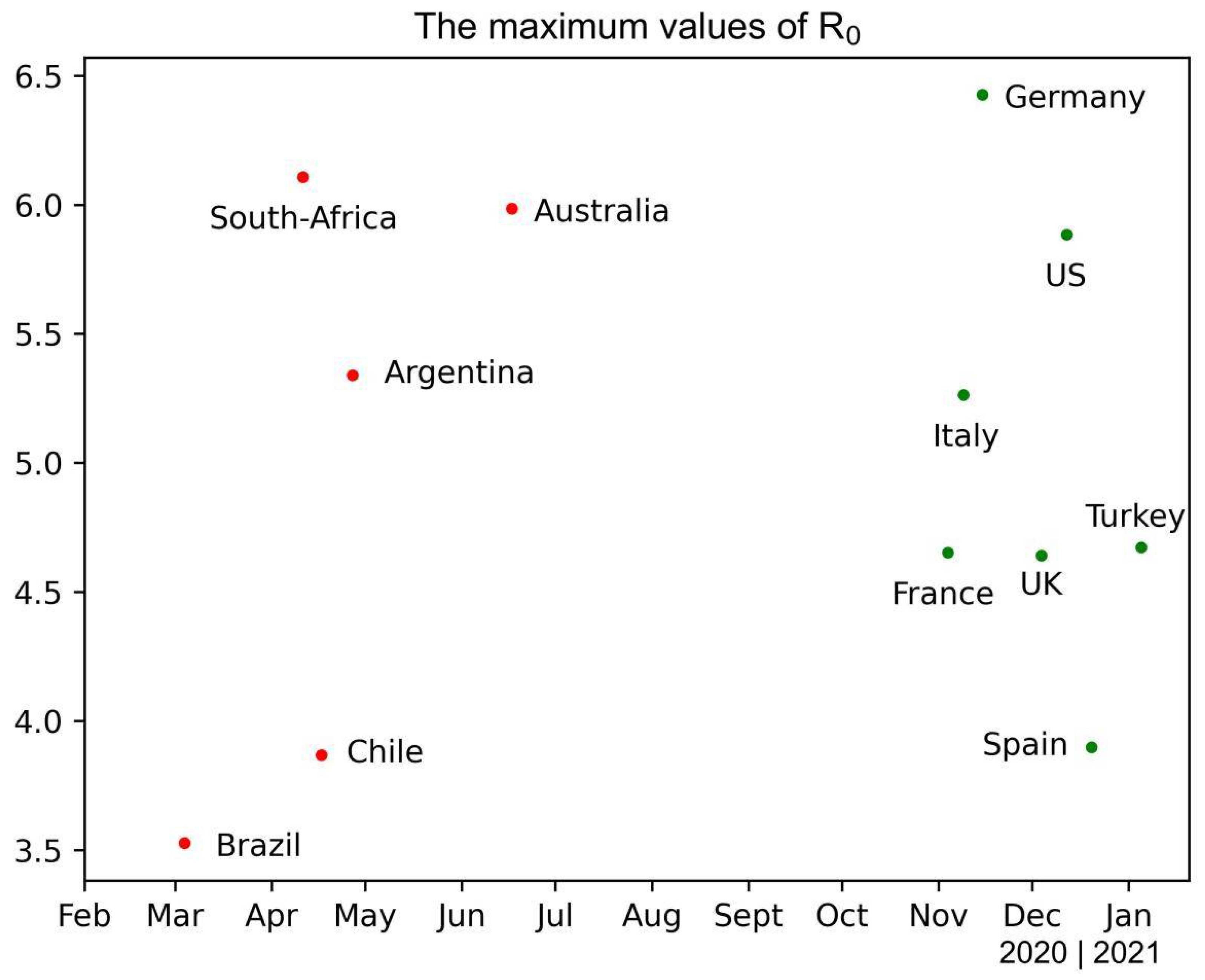
| Countries | A0 | A1 | Maximum Value (A1 + A0) | Minimum Value (A1 − A0) | |||||
|---|---|---|---|---|---|---|---|---|---|
| United States | 86 | 0.56 | 5.32 | 5.88 | 4.76 | 0.17 | 0.21 | 0.25 | 3.00 |
| France | 121 | 1.07 | 3.58 | 4.65 | 2.51 | 0.13 | 0.47 | 0.05 | 0.02 |
| Brazil | 14 | 0.84 | 2.69 | 3.53 | 1.85 | 0.32 | 0.50 | 0.07 | 0.70 |
| United Kingdom | 98 | 0.50 | 4.14 | 4.64 | 3.64 | 0.17 | 0.31 | 1.02 | 3.00 |
| Italy | 108 | 1.24 | 4.02 | 5.26 | 2.78 | 0.16 | 0.31 | 0.12 | 0.22 |
| Germany | 110 | 1.25 | 5.17 | 6.42 | 3.92 | 0.16 | 0.23 | 0.48 | 0.96 |
| Turkey | 71 | 1.82 | 2.85 | 4.67 | 1.02 | 0.14 | 0.79 | 0.08 | 0.02 |
| Australia | 274 | 1.10 | 4.88 | 5.99 | 3.78 | 0.09 | 0.23 | 0.47 | 0.11 |
| Spain | 66 | 0.63 | 3.27 | 3.90 | 2.64 | 0.23 | 0.40 | 0.54 | 0.05 |
| Argentina | 339 | 0.74 | 4.60 | 5.34 | 3.86 | 0.23 | 0.27 | 0.23 | 3.00 |
| South-Africa | 347 | 1.80 | 4.31 | 6.11 | 2.51 | 0.15 | 0.40 | 0.30 | 0.19 |
| Chile | 339 | 1.27 | 2.60 | 3.87 | 1.33 | 0.31 | 0.69 | 0.09 | 3.00 |
Publisher’s Note: MDPI stays neutral with regard to jurisdictional claims in published maps and institutional affiliations. |
© 2022 by the authors. Licensee MDPI, Basel, Switzerland. This article is an open access article distributed under the terms and conditions of the Creative Commons Attribution (CC BY) license (https://creativecommons.org/licenses/by/4.0/).
Share and Cite
Zheng, Y.; Wang, Y. How Seasonality and Control Measures Jointly Determine the Multistage Waves of the COVID-19 Epidemic: A Modelling Study and Implications. Int. J. Environ. Res. Public Health 2022, 19, 6404. https://doi.org/10.3390/ijerph19116404
Zheng Y, Wang Y. How Seasonality and Control Measures Jointly Determine the Multistage Waves of the COVID-19 Epidemic: A Modelling Study and Implications. International Journal of Environmental Research and Public Health. 2022; 19(11):6404. https://doi.org/10.3390/ijerph19116404
Chicago/Turabian StyleZheng, Yangcheng, and Yunpeng Wang. 2022. "How Seasonality and Control Measures Jointly Determine the Multistage Waves of the COVID-19 Epidemic: A Modelling Study and Implications" International Journal of Environmental Research and Public Health 19, no. 11: 6404. https://doi.org/10.3390/ijerph19116404