
A Comparison of Time-Series Predictions for Healthcare Emergency Department Indicators and the Impact of COVID-19

1
Transforming Systems, 8th Floor, 6 Mitre Passage, London SE10 0ER, UK
2
School of Computing & Mathematical Sciences, University of Greenwich, Park Row, Greenwich, London SE10 9LS, UK
*
Author to whom correspondence should be addressed.
Appl. Sci. 2021, 11(8), 3561; https://doi.org/10.3390/app11083561
Submission received: 5 November 2020
/
Revised: 18 March 2021
/
Accepted: 25 March 2021
/
Published: 15 April 2021
(This article belongs to the Special Issue Applied Machine Learning)
Abstract
:Featured Application
This application is being developed as part of a suite of tools used by the National Health Service (NHS) to analyse and predict pressure in resource management indicators (see transformingsystems.com for more details).
Abstract
Across the world, healthcare systems are under stress and this has been hugely exacerbated by the COVID pandemic. Key Performance Indicators (KPIs), usually in the form of time-series data, are used to help manage that stress. Making reliable predictions of these indicators, particularly for emergency departments (ED), can facilitate acute unit planning, enhance quality of care and optimise resources. This motivates models that can forecast relevant KPIs and this paper addresses that need by comparing the Autoregressive Integrated Moving Average (ARIMA) method, a purely statistical model, to Prophet, a decomposable forecasting model based on trend, seasonality and holidays variables, and to the General Regression Neural Network (GRNN), a machine learning model. The dataset analysed is formed of four hourly valued indicators from a UK hospital: Patients in Department; Number of Attendances; Unallocated Patients with a DTA (Decision to Admit); Medically Fit for Discharge. Typically, the data exhibit regular patterns and seasonal trends and can be impacted by external factors such as the weather or major incidents. The COVID pandemic is an extreme instance of the latter and the behaviour of sample data changed dramatically. The capacity to quickly adapt to these changes is crucial and is a factor that shows better results for GRNN in both accuracy and reliability.
1. Introduction
Across the world, healthcare systems are under stress and this has been hugely exacerbated by the COVID pandemic. Key Performance Indicators (KPIs), usually in the form of time-series data, are used to help manage that stress. Making reliable predictions of these indicators, particularly for emergency departments (ED), can help to identify pressure points in advance and also allows for scenario planning, for example, to optimise staff shifts and planning escalation actions.
According to Medway Foundation Trust (MFT), where the results of this study are applied, it is important to accurately forecast after exceptional events in their data, such as the pandemic, because forecasts are of increased importance at these critical moments. When the uncertainty level is greater, correct predictions may benefit their decision making more than usual (although models must also perform well in non-exceptional circumstances).
When analysing the healthcare systems, great significance has been placed on predicting patient arrivals in acute units, and in particular emergency department (ED) attendances and throughput. Typically, patients arrive at irregular intervals, often beyond the control of the hospital, and arrivals show strong seasonal and stochastic fluctuations driven by factors such as weather, disease outbreaks, day of the week and socio-demographic effects [1]. Accordingly, researchers use a variety of methods to predict ED visits over various periodic intervals, e.g., [2,3].
Furthermore, predicting KPIs in EDs can depend on several factors, e.g., [4,5]. Typically, EDs deal with a variety of life-threatening emergencies, arising from causes such as car accidents, disease, pollution, work-place hazards, aging, changing population, pandemics and many other sources. However, multivariate models usually consider only a small number of dependent/independent variables out of numerous possibilities, and in ED that can result in dangerous omissions. For example, variables that are not captured (especially those with high correlations, multi-variable correlation lags and high levels of noise) may drive multi-variate predictions of captured variables in the wrong direction [6].
For predictions of this type, a common approach is to auto-correlate the data. Since all the numerous variables have been an influence on the past values of the time-series under investigation, prediction models can use these data as a baseline to calculate future time-series values. Apart from this baseline, other variables, both dependent and independent, and represented by other indicators, may be included in the model by considering the covariance between them.
Accurate and reliable forecasts of various types of indicator can help to efficiently allocate key healthcare resources, including staff, equipment and vehicles, when and where they are most needed [2], and avoid allocating them at non-critical periods. This justifies considerable efforts to make reliable and accurate predictions of ED data to help hospital managers in making decisions about how to meet the expected healthcare demand effectively and in a timely fashion [1].
As a linear model, ARIMA can typically capture linear patterns in a time series efficiently, and so many studies adopt it either to evaluate relationships between variables, or use ARIMA forecasts as a benchmark against which to test the effectiveness of other models, e.g., [7].
This has been applied to ED data previously and as examples, Sun et al. [3], Afilal et al. [8], and Milner [9] have developed ARIMA models for forecasting hospital ED attendances and have verified the fitness of ARIMA, in that context, as a readily available tool for predicting ED workload. In particular, Milner [9] used ARIMA to forecast yearly patient attendances at EDs in the Trent region of the UK and found that the forecast for attendances was just 3 per cent away from the actual figure. Meanwhile, Sun et al. [3] were able to improve on the ARIMA results for daily patient attendances in Singapore General Hospital by incorporating other variables such as public holidays, periodicities and air quality.
Another option is to use proprietary models. One such, Prophet, is a forecasting model developed at Facebook Research, an R&D branch of the company. Taylor & Letham [10] observed that ARIMA forecasts can be prone to large trend errors, particularly when a change in trend occurs close to the cut-off period, and often fail to capture any seasonality. In experiments with Prophet, Taylor and Letham [10] predicted the daily number of Facebook events in a 30-day horizon with 25% more accuracy than ARIMA. The accurate prediction of these daily Facebook events, which are captured by an indicator with similar characteristics as some of the healthcare indicators, particularly in terms of in trend, seasonality and holidays, and which are at the heart of the Prophet model decomposition, motivated their use in this study.
Finally, a number of Machine Learning models are used to predict data, specifically for time-series processes, and in particular Neural Network variants have presented encouraging results for classification problems, e.g., [11,12]. In this study, after fitting models of LSTM (Long Short-Term Memory), RNN (Recurrent Neural Network) and RBN (Radial Basis Network), we present the results for the model found to best fit the data sample in our simulations, that is RBN, and in particular GRNN (Generalised Regression Neural Networks).
The rest of the paper is organised as follows: Section 2, Section 3 and Section 4 give more details of ARIMA, Prophet and GRNN, respectively. Section 5 describes the data and Section 6 gives details of how COVID has impacted on it. The main parts of the paper are Section 7 which describes the experimentation, and Section 8 that analyses those results. Finally, Section 9 presents conclusions and suggestions for further work.
2. Autoregressive Integrated Moving Average (ARIMA)
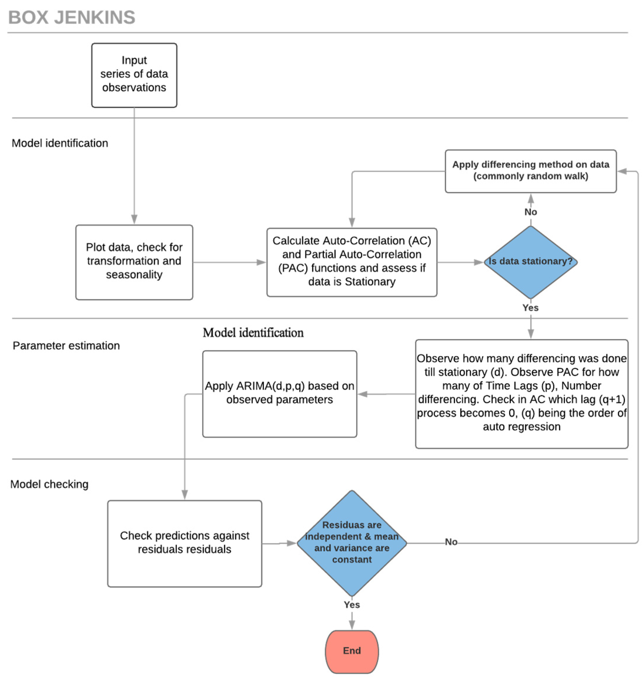
The Autoregressive Integrated Moving Average (ARIMA) model integrates Auto Regressive and Moving Average calculations. A basic requirement for predicting time-series with ARIMA is that the time-series should be stationary or, at the very least, trend-stationary [3,7]. A stationary series is one that has no trend, and where variations around the mean have a constant amplitude, e.g., [1,13,14]. Although ARIMA expects a stationary stochastic process as input, very few datasets are natively in such format, thus the use of differencing to “stationarise” is in the model identification stage [1,7] (Figure 1).
The ARIMA model has 3 key parameters (p, d, q), all non-negative integers: p is the order (the number of time lags) of the autoregressive model, d is the degree of differencing (the number of times the data have had past values subtracted if random walk is chosen), and q is the order of the moving-average model. The values for p, d, and q are defined by calculations and subsequent analysis and the process of fitting an ARIMA model, by calculating these parameters, is commonly known as the Box-Jenkins method [15].
The integration of the p autoregressive and q moving average terms, gives rise to the formula [15]:
where c represents a constant variable, error terms are generally assumed to be independent, uniformly distributed random variables, yt are previous observed values of the time-series and and are coefficients determined as part of the process.
Each indicator under analysis here has been through the three-stage ARIMA/Box-Jenkins iterative modelling approach (Figure 1):
- Model identification, to ensure that variables are stationary: if not, differencing methods such as random walk are applied, any seasonality is identified, and then AC (Auto Correlation) and PAC (Partial Auto Correlation) functions are plotted [16].
- Parameter estimation: using methods such as Non-linear Least Squares Estimation or Maximum Likelihood Estimation together with the outcome of the AC and PAC functions [16].
- Model checking, to test whether predictions now adhere to the requirements of a stationary univariate process: in particular, residuals must be independent of each other and within an acceptable range. Additionally, the mean and variance should be constant over the time. If the model is still inadequate, the iterative process returns to stage 1 and an alternative method for differencing is applied.
3. Prophet
Prophet is a forecasting model from Facebook Research. As discussed by Taylor & Letham, forecasting is a data science task, central to many activities within a large organization such as Facebook, and crucial for capacity planning and the efficient allocation of resources [10].
Prophet is motivated by the idea that not every prediction problem can be tackled using the same solution, and has been created with the aim of optimising business forecasting tasks encountered at Facebook that typically have some or all of the following characteristics [10]:
- Regular (hourly, daily, or weekly observations with at least a few months and preferably a year or more of history;
- Strong repeated “human-scale” seasonality (e.g., day of week or time of year);
- Significant holidays, often that occur at irregular intervals, but known in advance (e.g., Thanksgiving, the Super Bowl);
- Not too many missing observations or significant outliers;
- Historical trend changes (e.g., as a result of product launches or changes in logging procedures);
- Trends that include non-linear growth curves, e.g., natural limits or saturation levels.
- Unlike ARIMA models, the measurements do not need to be regularly spaced (stochastic process), thus Prophet also does not require time-series to be stationary.
Prophet uses a composite time-series model to predict y(t), with three main component, trend, seasonality, and holidays, that are combined as:
Here, g(t) is the trend function, s(t) models seasonal changes, and h(t) represents holidays, whilst represents an error term which is expected to be normally distributed [10].
3.1. Trend Model
Prophet’s main forecast component is the trend term, g(t), which defines how the time-series has developed previously and how it is expected to continue. Two choices are available for this trend function depending on the data characteristics: a Nonlinear Saturating Growth model, where the growth is non-linear and expected to saturate at a carrying capacity, and a Linear Model, where the rate of growth is stable [17].
In the case of the experiments in Section 7, the choice of trend function was determined automatically by Prophet.
3.2. Seasonality
Prophet also considers seasonal data patterns arising from similar behaviour repeated over several data intervals. To address this component of the model Prophet employs Fourier series’ to capture and model periodic effects [17].
This is very appropriate for the data under investigation which may exhibit multiple seasonal patterns. For example, hospital ED departments are typically busier every day between 5 p.m. and 8 p.m. from a variety of causes such as people suffering injuries when commuting, taking relatives to hospital after working hours, or injuries when exercising, etc. Meanwhile longer nested trends can arise as hospital EDs are usually busier in winter as compared with summer due to respiratory illness, slippery conditions, etc.
3.3. Holidays and Events
Holidays and special events provide a relatively significant, and normally predictable changes in time-series. Normally these do not have a regular periodic pattern (unlike, say, weekends) and thus the effects are not well modelled by a smooth cycle.
4. General Regression Neural Network (GRNN)
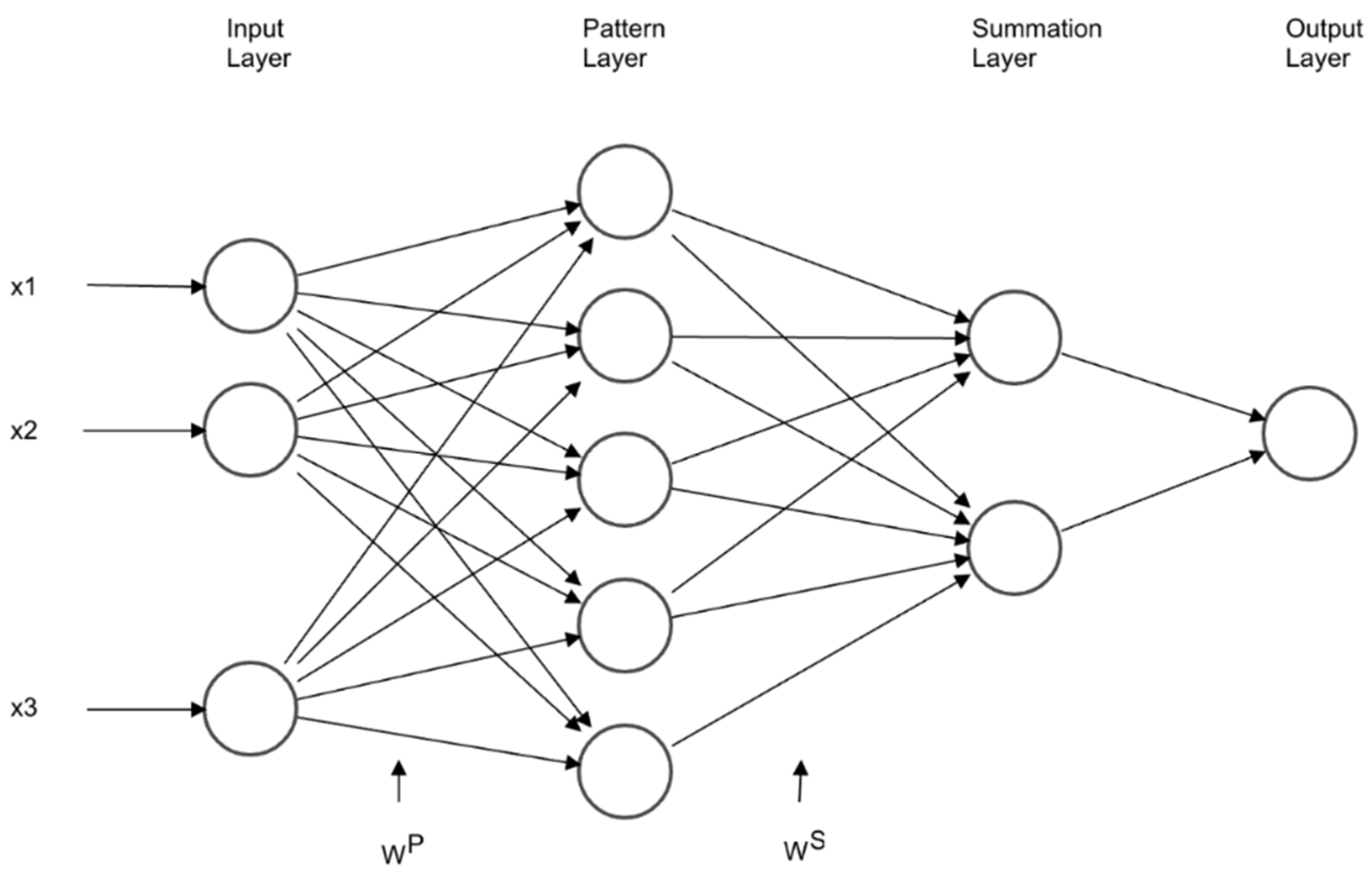
The General Regression Neural Network (GRNN) proposed by Specht [18] is a feed-forward neural network, responding to an input pattern by processing the input data from one layer to the next with no feedback paths. GRNN is a one-pass learning algorithm with a highly parallel structure. Even in the case a time-series has sparse observations with a non-stochastic process, the model outputs smooth transitions between resulting observations. The algorithmic form may be used for any regression problem provided that linearity is not justified.
The GRNN is considered a type of RBF (Radial Basis Function) neural network, that employs a fast, single pass learning. It consists of a hidden layer with RBF neurons. Typically, the hidden (Pattern) layer has the number of neurons similar to training examples. The center of a neuron is the linked training example, thus the output provides a measure of the closeness of the input vector to the training example. A subsequent summation layer is added to compute the results (Figure 2).
Normally, a neuron uses the multivariate Gaussian function [19].
where is the centre, the smoothing parameter and x the input vector.
Considering a training set of size n, patterns {…}, and their associated targets, {…}, the output is calculated in 2 stages, first the hidden layer produces weights representing levels of similarity of to training patterns:
The further away the training pattern is, the smaller the effect in the weight. The total sum of weights corresponds to 1, representing the proportional strength in the result.
The smoothing parameter , provides control on how many parameters are to be considered in the calculation and is an important part of model fitting, as it depends on the level of correlation and lags.
The second stage is the resulting calculation of future values :
The resulting calculation is nothing more than a weighted average of training targets.
4.1. Multi-Step Ahead Strategy
When predicting an hourly time-series of ED data, such as the Number of Patient Attendances, it is fair to expect to forecast a number of hours ahead, ideally every hour of the next seven days. For this a multi-step ahead strategy must be employed. There are two options, the MIMO (Multiple Input Multiple Output) strategy, and a Recursive strategy.
The MIMO strategy for predicting a series of future observations consists in employing training targets vectors with consecutive observations of the time-series, with the size of those vectors corresponding to the number of predicted observations desired.
The Recursive strategy is based in the one step ahead model as provided by the above equations. The model is applied recursively, matching the desired number of steps ahead, feeding predicted values as input variables. The recursive strategy was the option utilised in the simulations of GRNN in this study: the motivation was not to depend on training target vectors, as this can potentially demand frequent re-training.
4.2. Controlling Seasonality by Autoregressive Lags
The GRNN model does not contain an embedded seasonal parameter, but this can be addressed by the use of autoregressive lags, grouping correlated data into the training vector. The lag definition and the smoothing parameters can be indicated by the AC (Auto Correlation) and PAC (Partial Auto Correlation) functions as discussed in Section 2.
5. Data Description
The choice of the most valuable Emergency Department Key Performance Indicators (ED KPIs), with the intention of capturing pressure in an acute unit, is an inter-disciplinary issue. Input from healthcare professionals, particularly hospital managers, and data scientists, was sought for this study. However, the KPIs must be chosen from data that are already being captured and not every theoretically useful indicator may be readily available.
The four KPIs under analysis, chosen from those available, are shown in Table 1. These data have been provided by Medway Foundation Trust (MFT), located in Kent, South East England and, in particular, focuses on the MFT Hospital ED Acute Unit. The time-series frequency of all 4 the KPIs is hourly.
KPIs of this nature are key metrics in evaluating NHS performance and related KPIs used as targets. For example, the NHS Constitution sets out that a minimum of 95% of patients attending an A&E department should be admitted, transferred or discharged within 4 h of their arrival [20].
6. COVID Impact
The COVID pandemic has impacted UK society, and hence the KPI data, dramatically. The first government advice on social distancing was published on 12 March 2020, before a formal lockdown was announced on 23 March 2020, led to a huge reduction in consumer demand in certain sectors, closure of business and factories and disrupted supply chains [21].
In preparation for the pandemic, hospitals invested in expanding resources that were necessary to treat a high volume of patients with the infection, including respirators, PPE (Personal Protective Equipment), staff, protocols and treatments [22].
During March, NHS trusts rapidly re-designed their services on a large scale to release capacity for treating patients with COVID-19. This included discharging thousands to free up beds, postponing planned treatment, shifting appointments online where possible and redeploying staff, a process covered widely in the media. NHS England alone published more than 50 sets of guidance to hospital specialists for the treatment of non-COVID-19 patients during the pandemic [22].
The impact of such measures was easily observed in the data, simulations and results of this study. Due to the fact of the lockdown added to the fear of contracting COVID, the chosen KPIs had a sudden and dramatic reductions in absolute numbers, as fewer were going to the ED.
Not all prediction models reviewed in this paper were able to immediately account for the sudden changes of this nature and hence their accuracy and reliability dropped drastically. In particular immediately obvious inaccuracies in the models are due to the fact they mostly rely on auto-regressive and seasonal parameters of 6 to 8 weeks prior to the current time. Thus, it usually took 3 to 6 weeks for the models to learn and adapt to the change depending on the indicator. However, well-trained machine learning models present encouraging results, as can be seen below.
7. Simulations and Results
Simulations with the three presented forecasting models have been performed to compare the relative accuracy and reliability when applied to the four chosen indicators. ARIMA, traditionally the standard model for healthcare time-series predictions, is used as a benchmark.
Observing the ACF (Auto Correlation Function) and initial model training, a strong correlation was found by hour and weekday, so data have been classified by these parameters when applying the models. Further to the classification, it was observed that the autocorrelation of the data was stronger in the 8 weeks prior to the forecasting, as the residuals when utilizing this interval were the smallest in simulations. Summarizing, each prediction was calculated using a rolling actuals timeseries subset of the 8 previous observations, classified with a lag = 168.
The subset of 8 observations means that when applying GRNN, the size of the input layer was equal to 8, although the number is small, it presented smaller residuals than trials with sizes of input layer ranging from 12, 20 and 30, this is believed to be due to the higher correlation of the data observed in the ACF. The sigma parameter for the GRNN was chosen to be 0.3, which was found to be the best fit in preliminary experimentation.
Each model has been trained until its residuals were minimal in simulations, then parameters fixed and subsequently applied to the same rolling actuals time-series subset, of the same data source, with equal periods and frequency. Predictions were then compared with actual values and analysed for accuracy and reliability over the period from 1 January 2020 to the end of October 2020. Each prediction made is hourly and has an event horizon of h = 168 h, corresponding to predicting every hour for 7 days in advance.
The results are presented in a number of figures showing actual observed values, predictions and residuals and then analysed in Section 8.
7.1. Patients in Department
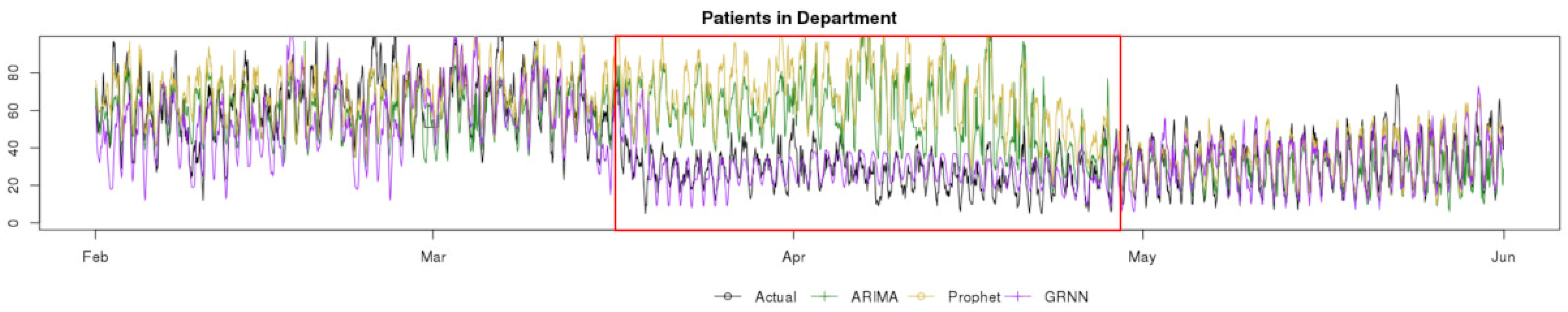
Figure 3 shows a comparison of actual observed data (in black) for the Patients in Department indicator compared with the ARIMA (green), Prophet (yellow) and GRNN (purple) predictions. Here, the red coloured square indicates the start of lockdown due to the COVID-19 pandemic. Three regions of the chart can be clearly distinguished (to the left, inside and to the right of the square) and indicate the normal number of Patients per hour in the Medway Foundation Trust ED before, during and after the lockdown, the sudden change, and the way data are slowly growing back in an apparent linear trend, from May to June. It is particularly interesting to see that ARIMA and Prophet overestimate their predictions for a five-week period, whilst GRNN is quick to adjust to the data ingress change. Another interesting observation is that the variance of the data is reduced after the lockdown, making the data easier to predict for all models. This is confirmed in the following figures which show predictions and actuals (top) and residuals (bottom) in more detail for each model.
In Figure 4 it can be observed that the ARIMA model predicts the Patients in Department time-series with a fair accuracy until the lockdown period, where the residuals negatively increase. Then, after five weeks the model learns the new levels and the residuals are again back to acceptable levels.
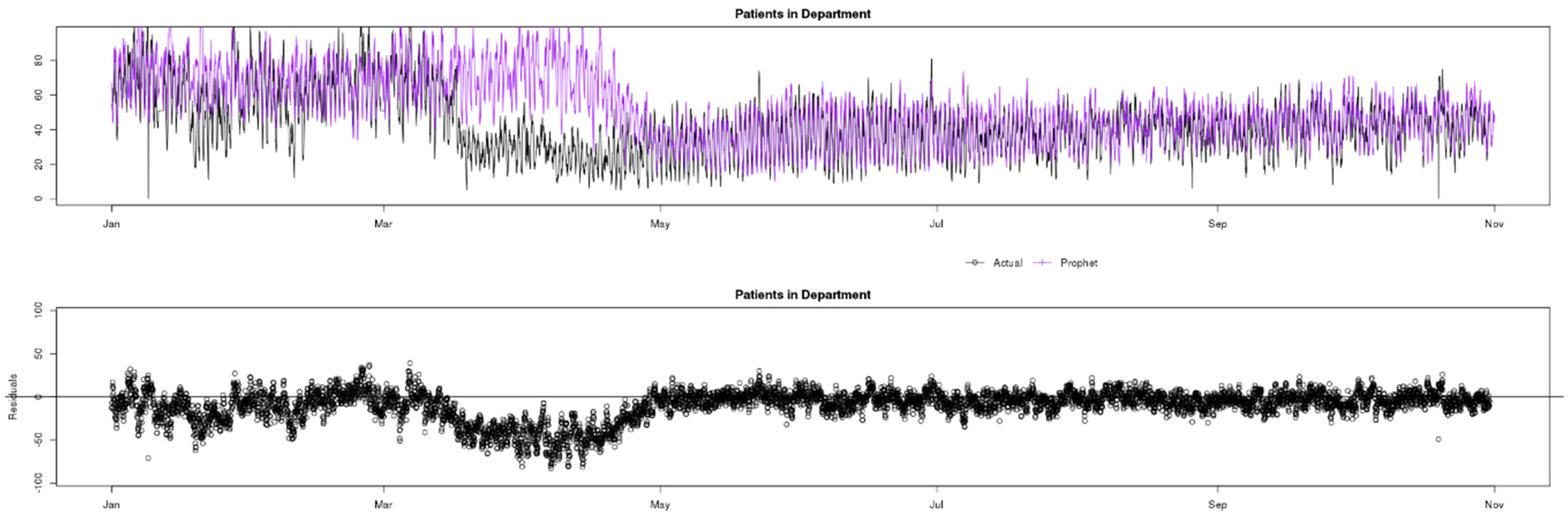
In Figure 5 it can be observed that Prophet, similar to ARIMA, predicts the Patients in Department indicator with fair accuracy until lockdown, during which the predictions are overestimated and the residuals increase by an even greater margin than ARIMA. However, after five weeks the model learns the new levels and the residuals are again back to acceptable levels.
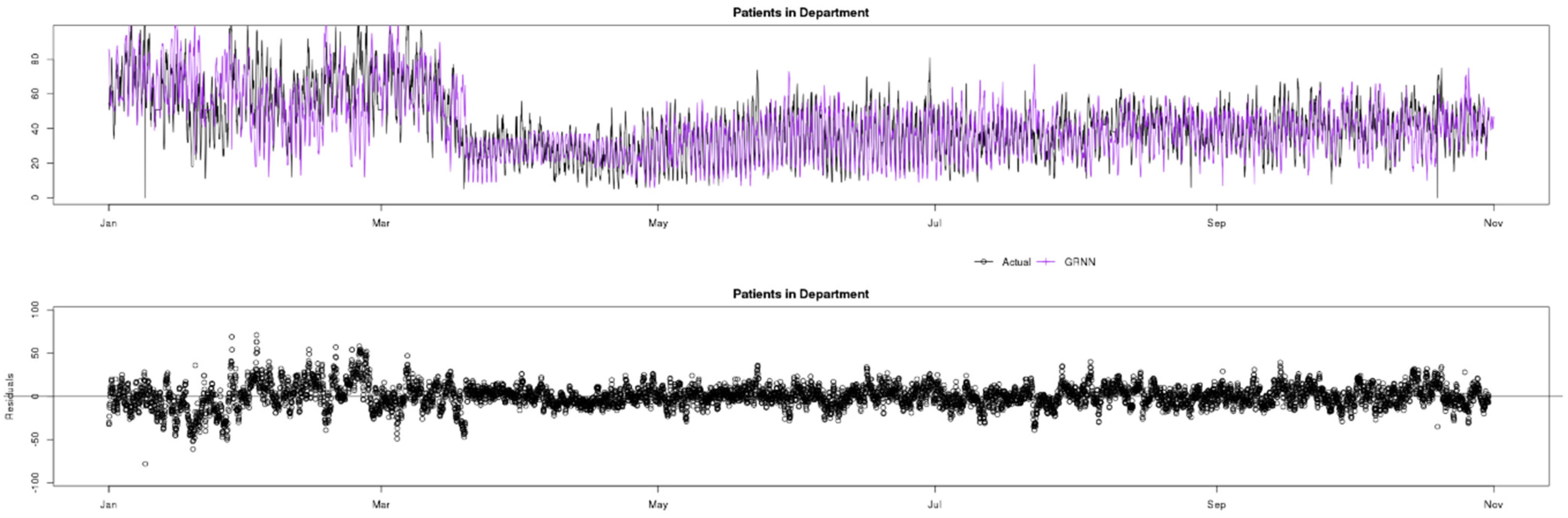
In Figure 6 it can be observed that GRNN, in contrast to the ARIMA and Prophet models, is able to quickly adapt to the change in observed values of Patients in Department due to COVID-19, keeping a good level of accuracy throughout the whole data sample.
7.2. Patient Attendances
Figure 7 shows a comparison of actual (black) data compared to ARIMA (green), Prophet (yellow) and GRNN (purple) predictions for the Patient Attendances indicator. The observed data contain a greater variance than Patients in Department, and this can alter the performance of prediction models. The COVID-19 pandemic caused a similar change in data behaviour to Patient Attendances, and GRNN was also the only model that quickly adapted to the change and accurately predicted the timeseries variables during this period.
The following figures breakdown this information and show the residual distributions.
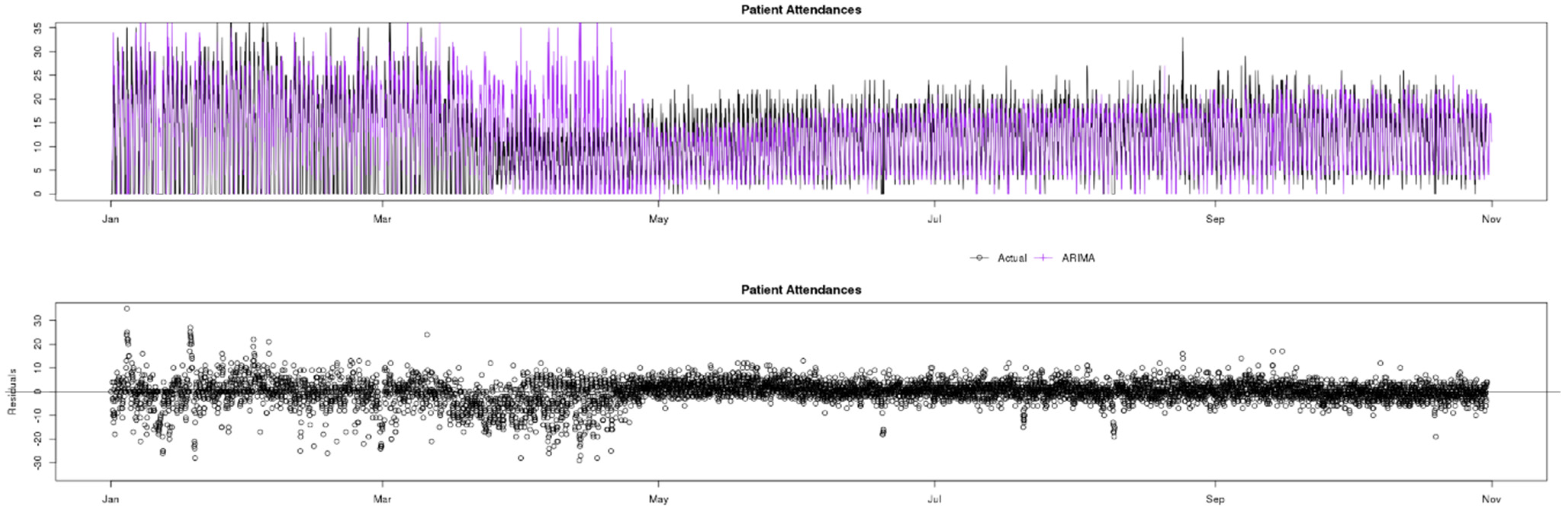
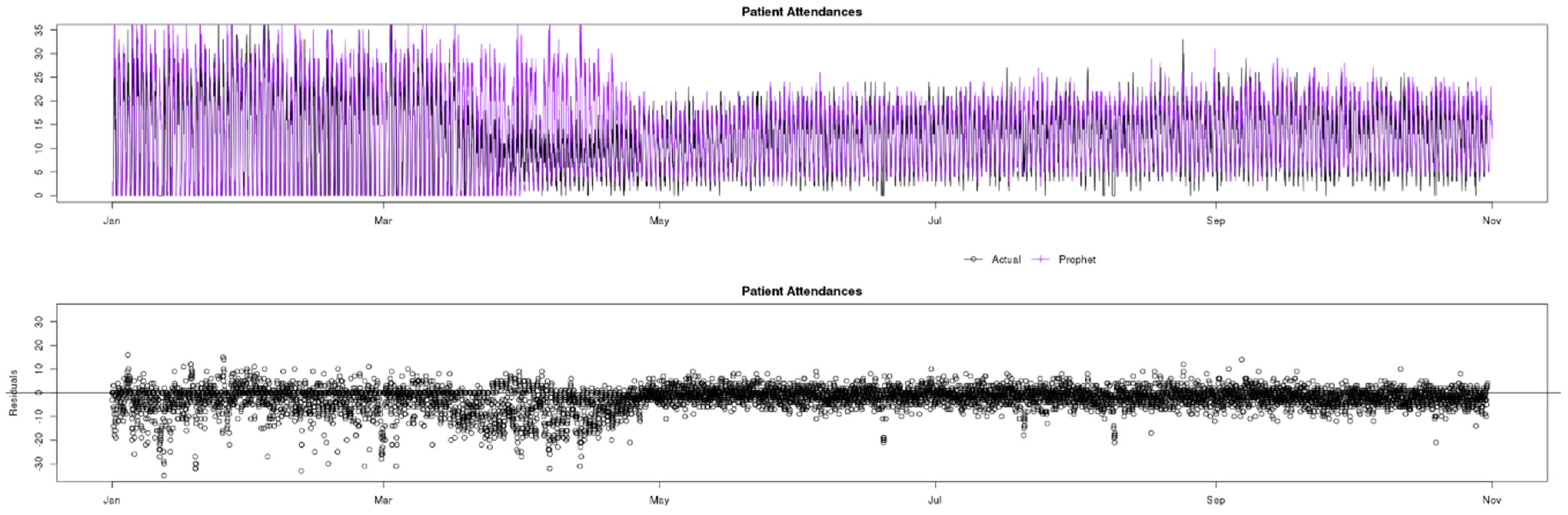
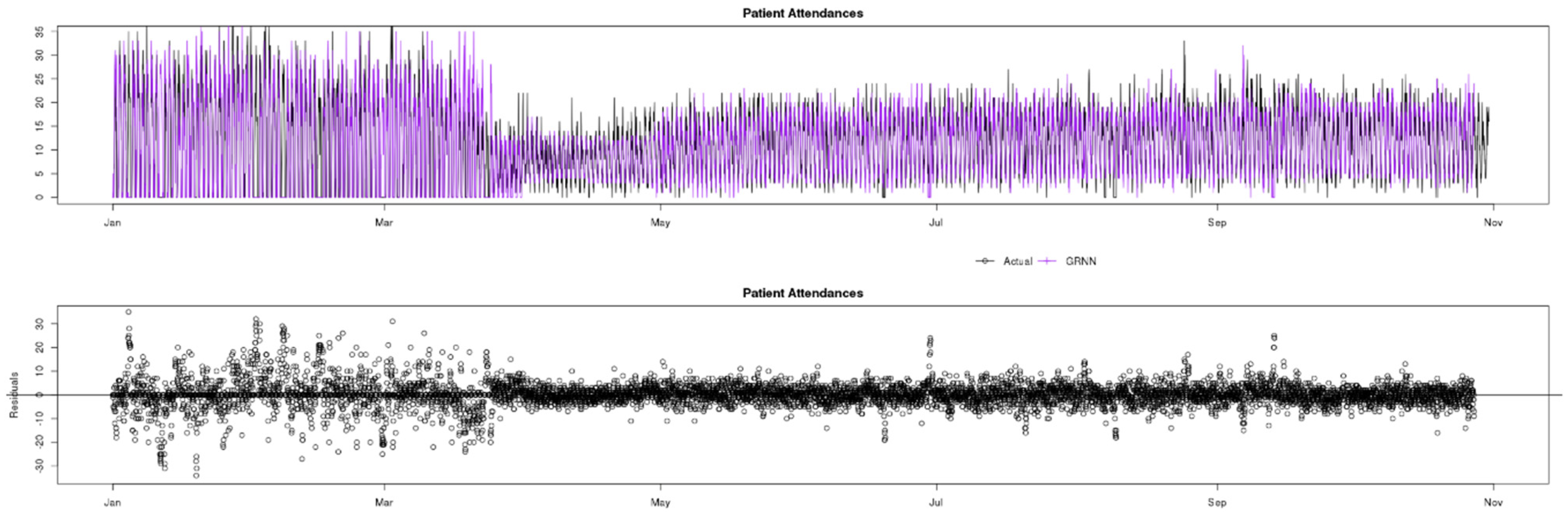
Observing the residuals charts at the bottom of Figure 8, Figure 9 and Figure 10, in the pre-lockdown phase ARIMA appears to be the best fit model as the residuals are concentrated closer to the x axis, whilst GRNN appears to have greater residuals and less accuracy in this phase. However, when the pandemic changed the data, GRNN was the only one of the three models to quickly adapt and predict with accuracy almost instantaneously, whilst both ARIMA and Prophet overestimated for approximately a 5 weeks period. In the post-lockdown phase, after all three models learned the new data behaviour, the performance is similar.
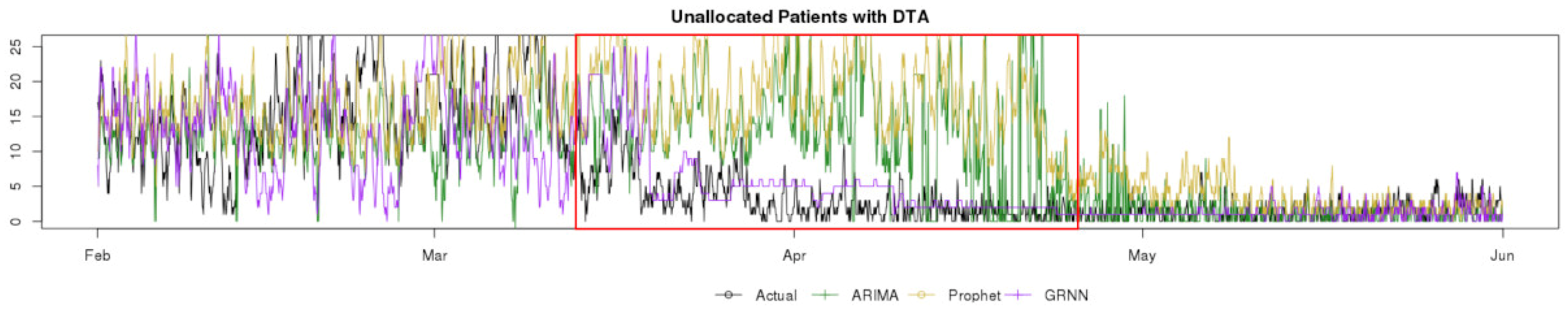
7.3. Unallocated Patients with DTA
Figure 11 shows a comparison of actual (black) data compared to ARIMA (green), Prophet (yellow) and GRNN (purple) predictions for the Unallocated Patients with DTA indicator. This indicator is perhaps the most challenging to predict in this study, as it includes a native and “variable” seasonal factor in that typically the decisions to admit patients are made in specific periods of the day, i.e., at the beginning of the doctors’ shifts, after their first meetings with patients. As doctors’ shifts commence at different times (unknown by the models), the lag factor of the seasonality is not constant, making the indicator somewhat unpredictable. This is the main reason residuals are typically greater than for other indicators.
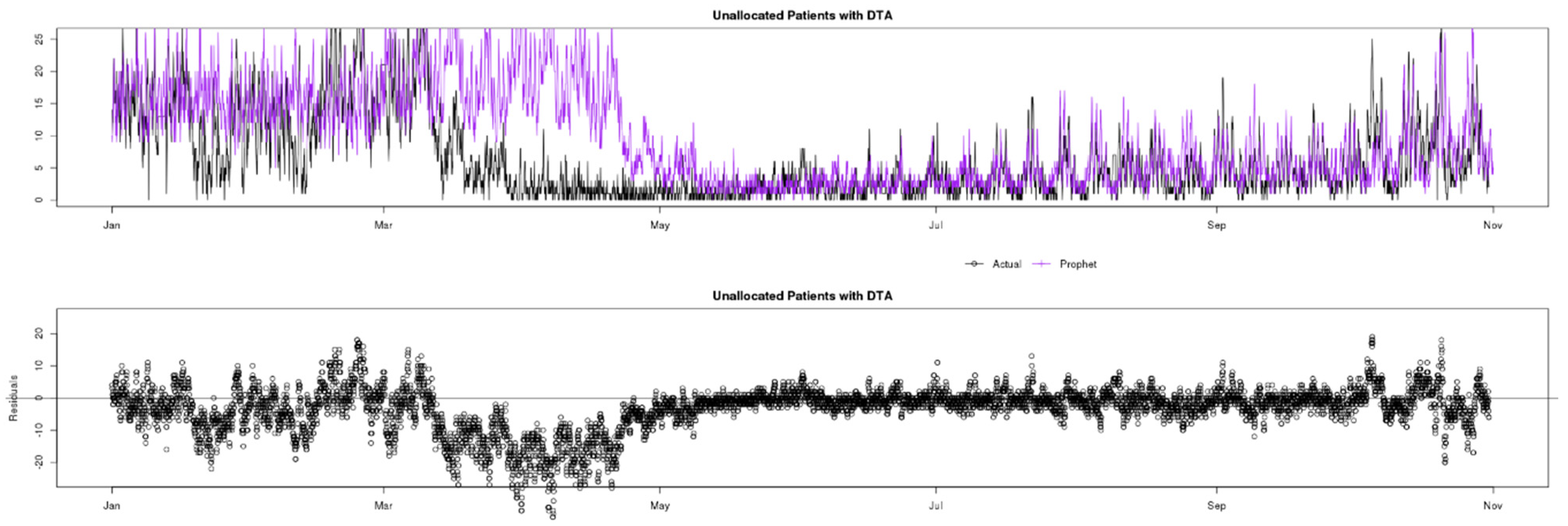
Looking at the residuals charts at the bottom of Figure 12, Figure 13 and Figure 14, the unpredictability mentioned can be clearly be observed by the high residuals in the pre-COVID phase for all three analysed models (ARIMA, Prophet and GRNN). During the lockdown affected period, as expected only GRNN predicts values reliably. In the post-lockdown learning period, all three models are able to reliably predict Unallocated Patients with DTA similarly, until October, when data change behaviour again, and ARIMA seems to explain the variables better.
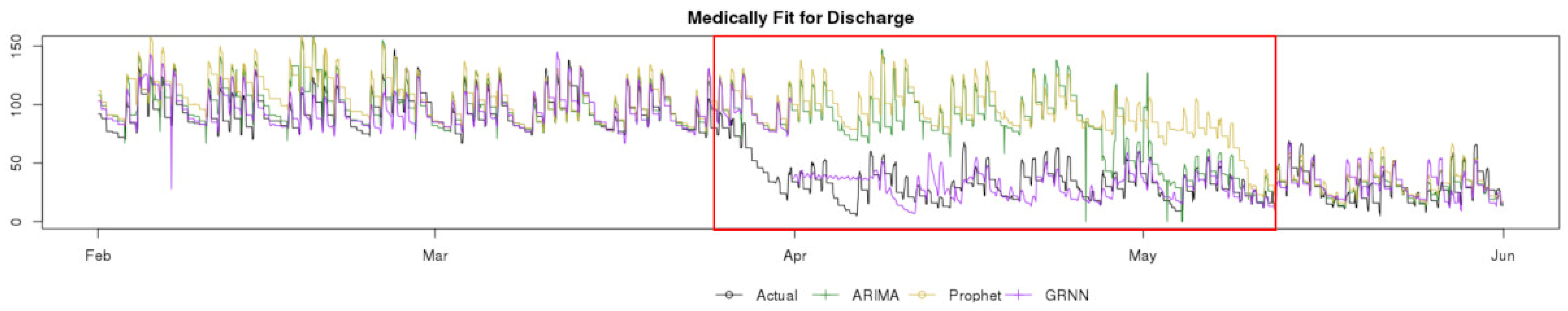
7.4. Medically Fit for Discharge
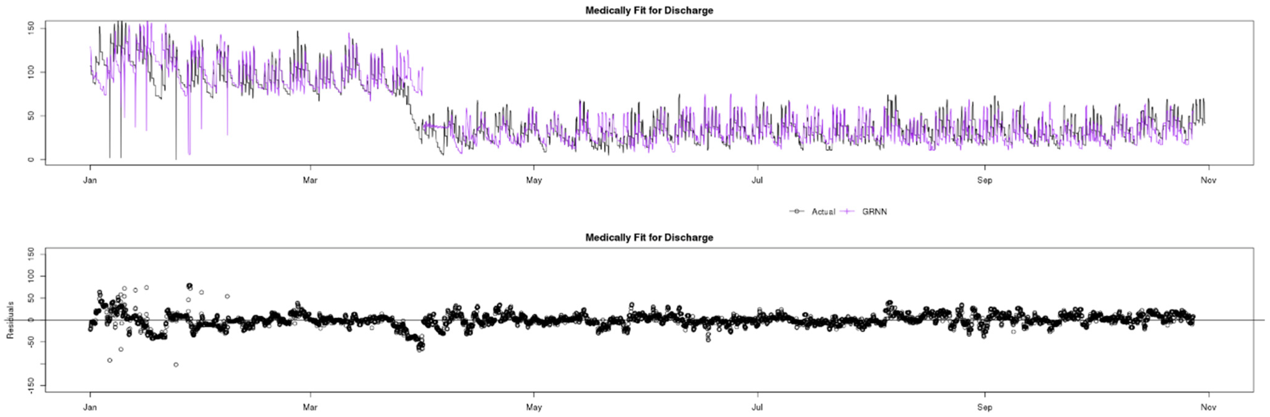
Figure 15 shows a comparison of actual (black) data compared to ARIMA (green), Prophet (yellow) and GRNN (purple) predictions for the Medically Fit for Discharge indicator. This indicator, unlike Unallocated Patients with DTA presents a very uniform seasonality and is thus a candidate for higher accuracy and reliability predictions. The reason is that doctors typically discharge patients at the same fixed times every day and this creates a very uniform lag factor, that is important to all auto-regressive processes. However, once again in the red square, it can be observed that GRNN is the only prediction model that can quickly adapt and provide reliable predictions during the lockdown period. Finally, there are some obvious outliers in the data, especially in February, but investigation has shown that these are due to data quality issues rather than unusual occurrences.
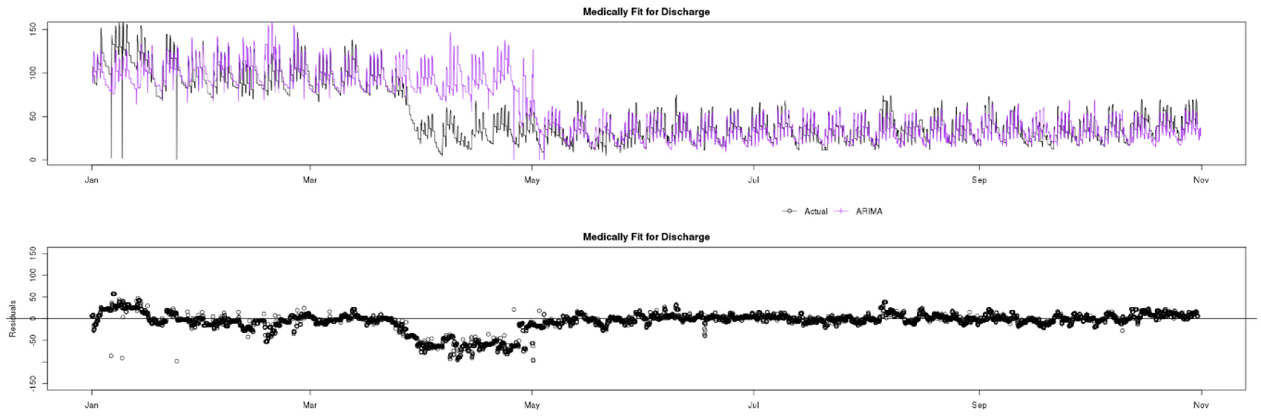
Once again, the residual charts in Figure 16, Figure 17 and Figure 18 show very small residuals for all three models, apart from the lockdown period, where GRNN is the only model that can adapt rapidly. This clear accuracy advantage is also highlighted by the red squares in Figure 3, Figure 7, Figure 11 and Figure 15. This may be dependent on the training, especially the size of the input layer, which, although the same for all models (8), by being relatively small may benefit GRNN, when the data change behaviour, and allow it a more agile response.
Finally, in the prediction chart of Figure 18, a few GRNN predictions are missing, and this is due to the model being sensitive to missing input of actual observations in this indicator time-series.
8. Reliability and Accuracy Analysis
Time-series predictions are commonly evaluated by looking at the “residuals”, as shown above, which are typically measured as the difference between actual values and predictions, often using the root mean squared error (RMSE).
8.1. Analysis
When emphasizing the importance of relevant measurements in evaluation of forecasting models, Krollner et al., 2010 [23] stated that over 80% of the papers reported that their model outperformed the benchmark model. However, most analysed studies do not consider real world constraints like trading costs and slippage. In this study, for the data presented, the residual analysis has been under discussion, as the usual measurements do not necessarily capture the quality of the time series forecasting in an Emergency Department if considering the applied science aspect, with real-world constraints. In particular, when analysing the environment of an ED, it is often more important to have approximated values constantly close, or within a certain threshold of the actuals, rather than keeping a low perceptual average RMSE.
To understand this, consider a situation where the average RMSE is low but exhibits occasional spikes. In an ED situation a spike corresponds to high unpredicted demand, such as a sudden large influx of patients, and may have dangerous clinical outcomes for patients if resource capacity is significantly exceeded on those occasions. A prediction which is less accurate on average, but which exhibits fewer spikes in RMSE is much preferred as it predicts changing demand more reliably, even if it is not always exact.
For this reason, in the analysis below (Table 2) every simulation contains confidence bands and accuracy metrics which provide a more readable measure for healthcare professionals (following discussions) to compare predictions. Thus “Very good” predictions have residuals that are no further than 15% of the actual mean away from the actual counterpart, “Good” are within 15–25%, “Regular” are within 25–40% of the mean, and any prediction with residual above 40% of the actual mean is considered “Unreliable”. Accordingly, all predictions that turned out to be within 40% of the actual values are classed as “Reliable” and overall “Reliability” (i.e., the total percentage of “Very good”, “Good” and “Regular” predictions) is used as a summary metric.
In addition, the average RMSE is also provided (Table 3) for each model and indicator, as the most neutral statistical residual measurement, even though, for the reasons outlined above, it may not the best fit for the ED environment.
In both cases, green highlighting indicates the model with the best results.
8.2. Discussion
As can be seen, and as already previewed above, the machine learning technique GRNN usually provides the best results for this dataset and usually outperforming ARIMA, which is traditionally used for predicting ED indicators. However, ARIMA usually comes a close second and actually outperforms GRNN for the Patient Attendances, probably due to the very high variance in this indicator.
The relative performance is heavily impacted by the ability of GRNN to adapt rapidly to sudden dramatic changes in the data trends and for more stable time-series data, the performance of all three is likely to be closer.
The COVID-19 pandemic drove just such a change and strongly altered the behaviour of ED indicators, which then presented a challenge to the purely autoregressive models represented by ARIMA and Prophet, which rely solely on abstractions of previous values. GRNN was able to adapt to the change in data patterns promptly, resulting in closer predictions during this change period for all 4 indicators, as seen in Section 7. In addition, when analysing the entire 10 months of data for reliability (Table 2) and accuracy (Table 3), GRNN was the best fit model for 3 out of the 4 indicators, as seen in Section 8.
Although the difference in both accuracy and reliability are evident and relevant, data analysis suggests that outside of the pandemic period, the improvements in accuracy and reliability are reduced to slim margins. Hence, further simulations with different KPIs and data sample periods are necessary to further validate the findings of this study.
9. Conclusions
The main conclusion of this paper is that prediction of Emergency Department (ED) indicators can be improved by using machine learning models such as GRNN in comparison to traditional models such as ARIMA, particularly when sudden changes are observed in the data.
Indeed, it may be the case that ARIMA is better overall when indicators are very stable and so the proposed extension of this study is aimed at creating hybrid predictions, mixing observed predictions of ARIMA, GRNN, and possibly even Prophet, into a mixed time-series forecasting model, based on the short-term seasonal accuracy factors achieved by each model.
Author Contributions
Conceptualization, all authors; methodology, D.D.; software, D.D.; investigation, D.D.; data curation, D.D.; writing—original draft preparation, D.D.; writing—review and editing, C.W. and N.R.; visualization, D.D.; supervision, C.W. and N.R.; funding acquisition, C.W. All authors have read and agreed to the published version of the manuscript.
Funding
This research was partially funded by an Innovate UK Knowledge Transfer Partnership, KTP10507.
Data Availability Statement
Restrictions apply to the availability of these data. Data was obtained from Transforming Systems and are available from the D.D. subject to the permission of Transforming Systems.
Conflicts of Interest
The authors declare no conflict of interest.
References
- Luo, L.; Luo, L.; Zhang, X.; He, X. Hospital daily outpatient visits forecasting using a combinatorial model based on ARIMA and SES models. BMC Health Serv. Res. 2017, 17, 469. [Google Scholar] [CrossRef] [PubMed] [Green Version]
- Permanasari, E.; Hidayah, I.; Bustoni, I.A. SARIMA (Seasonal ARIMA) implementation on time series to forecast the number of Malaria incidence. In Proceedings of the 2013 International Conference on Information Technology and Electrical Engineering (ICITEE), Yogyakarta, Indonesia, 7–8 October 2013; pp. 203–207. [Google Scholar] [CrossRef]
- Sun, Y.; Heng, B.H.; Seow, Y.T.; Seow, E. Forecasting daily attendances at an emergency department to aid resource planning. BMC Emerg. Med. 2009, 9, 1. [Google Scholar] [CrossRef] [PubMed] [Green Version]
- Jones, S.S.; Evans, R.S.; Allen, T.L.; Thomas, A.; Haug, P.J.; Welch, S.J.; Snow, G.L. A multivariate time series approach to modeling and forecasting demand in the emergency department. J. Biomed. Inform. 2009, 42, 123–139. [Google Scholar] [CrossRef] [PubMed] [Green Version]
- Kunst, R.; Neusser, K. A forecasting comparison of some var techniques. Int. J. Forecast. 1986, 2, 447–456. [Google Scholar] [CrossRef]
- Aboagye-Sarfo, P.; Mai, Q.; Sanfilippo, F.M.; Preen, D.B.; Stewart, L.M.; Fatovich, D.M. A comparison of multivariate and univariate time series approaches to modelling and forecasting emergency department demand in Western Australia. J. Biomed. Inform. 2015, 57, 62–73. [Google Scholar] [CrossRef] [PubMed] [Green Version]
- Zhu, T.; Luo, L.; Zhang, X.; Shi, Y.; Shen, W. Time-Series Approaches for Forecasting the Number of Hospital Daily Discharged Inpatients. IEEE J. Biomed. Health Inform. 2017, 21, 515–526. [Google Scholar] [CrossRef] [PubMed]
- Afilal, M.; Yalaoui, F.; Dugardin, F.; Amodeo, L.; Laplanche, D.; Blua, P. Forecasting the Emergency Department Patients Flow. J. Med. Syst. 2016, 40, 175. [Google Scholar] [CrossRef] [PubMed]
- Milner, P.C. Ten-year follow-up of arima forecasts of attendances at accident and emergency departments in the Trent region. Stat. Med. 1997, 16, 2117–2125. [Google Scholar] [CrossRef]
- Taylor, S.J.; Letham, B. Forecasting at Scale. PeerJ Prepr. 2017, 5, 25. [Google Scholar] [CrossRef]
- Bani-Hani, D.; Khasawneh, M. A Recursive General Regression Neural Network (R-GRNN) Oracle for classification problems. Expert Syst. Appl. 2019, 135, 273–286. [Google Scholar] [CrossRef]
- Apaydin, H.; Feizi, H.; Sattari, M.T.; Colak, M.S.; Shamshirband, S.; Chau, K.W. Comparative analysis of recurrent neural network architectures for reservoir inflow forecasting. Water 2020, 12, 1500. [Google Scholar] [CrossRef]
- Xu, Q.; Tsui, K.-L.; Jiang, W.; Guo, H. A Hybrid Approach for Forecasting Patient Visits in Emergency Department. Qual. Reliab. Engng. Int. 2016, 32, 2751–2759. [Google Scholar] [CrossRef]
- Channouf, N.; L’Ecuyer, P.; Ingolfsson, A.; Avramidis, A.N. The application of forecasting techniques to modeling emergency medical system calls in Calgary, Alberta. Health Care Manag. Sci. 2007, 10, 25–45. [Google Scholar] [CrossRef] [PubMed]
- Box, G.E.P.; Jenkins, G.M. Time Series Analysis: Forecasting and Control, 2nd ed.; University of Michigan, Holden-Day: Ann Arbor, MI, USA, 1976. [Google Scholar]
- Vandaele, W. Applied Time Series and Box-Jenkins Models, 2nd ed.; Academic Press, Inc.: San Diego, CA, USA, 1983. [Google Scholar]
- McCoy, T.H.; Pellegrini, A.M.; Perlis, R.H. Assessment of Time-Series Machine Learning Methods for Forecasting Hospital Discharge Volume. JAMA Netw. Open 2018, 1, e184087. [Google Scholar] [CrossRef] [PubMed]
- Specht, D.F. Probabilistic Neural Networks and General Regression Neural Networks; Palo Alto: Santa Clara, CA, USA, 1995; Volume 67. [Google Scholar]
- Al-Mahasneh, J.; Anavatti, S.G.; Garratt, M.A.; Pratama, M. Evolving General Regression Neural Networks Using Limited Incremental Evolution for Data-Driven Modeling of Non-Linear Dynamic Systems. In Proceedings of the 2018 IEEE Symposium Series on Computational Intelligence, SSCI 2018, Bangalore, India, 18–21 November 2018; pp. 335–341. [Google Scholar] [CrossRef]
- Fisher, E.; O’dowd, N.C.; Dorning, H.; Keeble, E.; Kossarova, L. Quality at a Cost. 2016. Available online: http://www.qualitywatch.org.uk/sites/files/qualitywatch/field/field_document/QWannualstatement2016%28final%29WEB.pdf (accessed on 19 February 2018).
- Stephens, M.; Cross, S.; Luckwell, G. Coronavirus and the Impact on Output in the UK Economy. Office for National Statistics. 2020; pp. 1–29. Available online: https://www.ons.gov.uk/economy/grossdomesticproductgdp/articles/coronavirusandtheimpactonoutputintheukeconomy/april2020 (accessed on 31 October 2020).
- Thorlby, R.; Tinson, A.; Kraindler, J. COVID-19: Five Dimensions of Impact|The Health Foundation. No. April. 2020, pp. 1–20. Available online: https://www.health.org.uk/news-and-comment/blogs/covid-19-five-dimensions-of-impact (accessed on 31 October 2020).
- Krollner, B.; Vanstone, B.; Finnie, G. Financial time series forecasting with machine learning techniques: A survey. In Proceedings of the 8th European Symposium on Artificial Neural Networks, ESANN 2010, Bruges, Belgium, 28–30 April 2010; pp. 25–30. [Google Scholar]
Figure 1.
The Box-Jenkins/ARIMA iterative fitting process.

Figure 2.
Schematic diagram of generalized regression neural networks (GRNN).

Figure 3.
Comparison of Actuals, ARIMA, Prophet and GRNN, February 2020–June 2020.

Figure 4.
Comparison of Actual and ARIMA with residual distribution chart, January 2020–November 2020.
Figure 4.
Comparison of Actual and ARIMA with residual distribution chart, January 2020–November 2020.

Figure 5.
Comparison of Actual and Prophet with residual distribution chart, January 2020–November 2020.
Figure 5.
Comparison of Actual and Prophet with residual distribution chart, January 2020–November 2020.

Figure 6.
Comparison of Actual and GRNN with residual distribution chart, January 2020–November 2020.
Figure 6.
Comparison of Actual and GRNN with residual distribution chart, January 2020–November 2020.

Figure 7.
Comparison of Actuals, ARIMA, Prophet and GRNN, February 2020–June 2020.

Figure 8.
Comparison of Actual and ARIMA with residual distribution chart, January 2020–November 2020.
Figure 8.
Comparison of Actual and ARIMA with residual distribution chart, January 2020–November 2020.

Figure 9.
Comparison of Actual and Prophet with residual distribution chart, January 2020–November 2020.
Figure 9.
Comparison of Actual and Prophet with residual distribution chart, January 2020–November 2020.

Figure 10.
Comparison of Actual and GRNN with residual distribution chart, January 2020–November 2020.
Figure 10.
Comparison of Actual and GRNN with residual distribution chart, January 2020–November 2020.

Figure 11.
Comparison of Actuals, ARIMA, Prophet and GRNN, February 2020–June 2020.

Figure 12.
Comparison of Actual and ARIMA with residual distribution chart, January 2020–November 2020.
Figure 12.
Comparison of Actual and ARIMA with residual distribution chart, January 2020–November 2020.

Figure 13.
Comparison of Actual and Prophet with residual distribution chart, January 2020–November 2020.
Figure 13.
Comparison of Actual and Prophet with residual distribution chart, January 2020–November 2020.

Figure 14.
Comparison of Actual and GRNN with residual distribution chart, January 2020–November 2020.
Figure 14.
Comparison of Actual and GRNN with residual distribution chart, January 2020–November 2020.

Figure 15.
Comparison of Actuals, ARIMA, Prophet and GRNN, February 2020–June 2020.

Figure 16.
Comparison of Actual and ARIMA with residual distribution chart, January 2020–November 2020.
Figure 16.
Comparison of Actual and ARIMA with residual distribution chart, January 2020–November 2020.

Figure 17.
Comparison of Actual and Prophet with residual distribution chart, January 2020–November 2020.
Figure 17.
Comparison of Actual and Prophet with residual distribution chart, January 2020–November 2020.

Figure 18.
Comparison of Actual and GRNN with residual distribution chart, January 2020–November 2020.
Figure 18.
Comparison of Actual and GRNN with residual distribution chart, January 2020–November 2020.


Table 1.
Key Performance Indicator Descriptions.
| Key Performance Indicator | Abbreviation | Description |
|---|---|---|
| Patients in Department | PD | Hourly average number of patients waiting to be seen in the ED (hourly) |
| Patient Attendances | PA | Hourly total number of patients with major injuries attending the ED |
| Unallocated Patients with DTA | UP | Number of patients that have been attended, not discharged, but waiting to be admitted to the hospital, thus occupying resources |
| Medically Fit for Discharge | MD | Total number of patients who have attended, and do not need further treatment |
Table 2.
Reliability comparison of ARIMA, Prophet and GRNN.
| Confidence Bands Data Distribution | ||||
|---|---|---|---|---|
| Residual Quality | ARIMA | Prophet | GRNN | |
| Patients in Department | Very good | 48.8% | 43.5% | 48.9% |
| Good | 16.4% | 16.2% | 19.2% | |
| Regular | 14.6% | 15.1% | 16.3% | |
| Unreliable | 20.2% | 25.2% | 15.6% | |
| Reliability | 79.8% | 74.8% | 84.4% | |
| Patient Attendances | Very good | 53.5% | 50.0% | 53.3% |
| Good | 13.0% | 12.0% | 12.4% | |
| Regular | 15.7% | 15.8% | 15.0% | |
| Unreliable | 17.8% | 22.2% | 18.3% | |
| Reliability | 82.2% | 77.8% | 80.7% | |
| Unallocated Patients with DTA | Very good | 32.1% | 28.7% | 36.2% |
| Good | 15.7% | 15.0% | 16.0% | |
| Regular | 10.5% | 11.6% | 11.1% | |
| Unreliable | 41.7% | 45.0% | 36.7% | |
| Reliability | 58.3% | 55.0% | 63.3% | |
| Medically Fit for Discharge | Very good | 53.5% | 44.0% | 53.4% |
| Good | 19.3% | 17.4% | 22.3% | |
| Regular | 10.7% | 14.6% | 13.1% | |
| Unreliable | 16.4% | 24.1% | 10.2% | |
| Reliability | 83.5% | 76.0% | 88.8% | |
Table 3.
Accuracy comparison of ARIMA, Prophet and GRNN.
| RMSE (Root Mean Square Deviation) | |||
|---|---|---|---|
| ARIMA | Prophet | GRNN | |
| Patients in Department | 18.1091 | 21.5031 | 17.7061 |
| Patient Attendances | 7.1002 | 8.8217 | 7.5965 |
| Unallocated Patients with DTA | 6.6968 | 8.1521 | 6.2153 |
| Medically Fit for Discharge | 35.1270 | 39.2894 | 34.3455 |
Publisher’s Note: MDPI stays neutral with regard to jurisdictional claims in published maps and institutional affiliations. |
© 2021 by the authors. Licensee MDPI, Basel, Switzerland. This article is an open access article distributed under the terms and conditions of the Creative Commons Attribution (CC BY) license (https://creativecommons.org/licenses/by/4.0/).
Share and Cite
MDPI and ACS Style
Duarte, D.; Walshaw, C.; Ramesh, N. A Comparison of Time-Series Predictions for Healthcare Emergency Department Indicators and the Impact of COVID-19. Appl. Sci. 2021, 11, 3561. https://doi.org/10.3390/app11083561
AMA Style
Duarte D, Walshaw C, Ramesh N. A Comparison of Time-Series Predictions for Healthcare Emergency Department Indicators and the Impact of COVID-19. Applied Sciences. 2021; 11(8):3561. https://doi.org/10.3390/app11083561
Chicago/Turabian StyleDuarte, Diego, Chris Walshaw, and Nadarajah Ramesh. 2021. "A Comparison of Time-Series Predictions for Healthcare Emergency Department Indicators and the Impact of COVID-19" Applied Sciences 11, no. 8: 3561. https://doi.org/10.3390/app11083561
Note that from the first issue of 2016, this journal uses article numbers instead of page numbers. See further details here.