1. Introduction
In response to the COVID-19 pandemic, there have been substantial reductions in many activities (e.g., driving, manufacturing, goods movement) that generate ozone and fine particulate matter (PM2.5) precursor emissions across the world. This has resulted in a real-world experiment of a sudden reduction in emissions that allows an assessment of how air quality responded to the reductions in emissions. Researchers seized the opportunity to study changes in air quality due to the COVID-19 pandemic, and numerous studies have been performed.
Seven months into the pandemic, Gkatzelis et al. [
1] reviewed the scientific literature of accepted peer-reviewed journals of over 200 papers that studied air quality changes during the pandemic. Many of the studies focused on the analysis of ground-based and/or satellite observations and reported a range of findings depending on study parameters: period, global geographic region, urban versus rural focus, primary versus secondary pollutants, degree of spatial aggregation, and consideration of confounding factors such as long-term trends and/or meteorological influences. However, despite these differences, consistent patterns have emerged. For example, Bekbulat et al. [
2] considered evidence from U.S. regulatory monitors and found that, in general, concentrations of ozone (O
3) and nitrogen dioxides (NOx) were lowered, but the reduction was modest and transient. Their findings are important on regional scales but, because they spatially aggregated data, important local scale variations (e.g., within the South Coast Air Basin (SoCAB) of California) may be obscured in their analysis. Fu et al. [
3] considered the Air Quality Index (AQI) in 20 major cities worldwide and found substantially decreased NO
2 concentrations and smaller, mixed impacts on ozone concentrations from COVID-19 lockdowns. For Los Angeles, they found lower NO
2 AQI but no noticeable effect on ozone AQI during their study period of 19 March–7 May 2020. Goldberg et al. [
4] utilized TROPOMI satellite data to disentangle the impact of the COVID-19 lockdowns on urban NO
2 from natural variability and found that, after accounting for meteorology, NO
2 reductions were between 9.2% and 43.4% among 20 cities in North America, and approximately 33% in Los Angeles from 15 March to 30 April 2020. Venter et al. [
5] utilized TROPOMI satellite data and ground-based observations and concluded that lockdown events have reduced the population-weighted concentration of nitrogen dioxide and particulate matter levels by about 60% and 31% in 34 countries, with mixed effects on ozone during lockdown dates up to 15 May 2020. Campbell et al. [
6] evaluated the impacts of the COVID-19 lockdowns on emissions and ozone air quality by using observational data and the National Air Quality Forecasting Capability (NAQFC) air quality modeling system, which utilizes CMAQ at 12 km resolution. Their study included the entire U.S. and evaluated the period March–September 2020. They found variable impacts on maximum daily 8-hr average (MDA8 ozone concentrations across the U.S., including widespread decreases in rural regions but also localized increases near some of the highly populated urban areas
The impacts of COVID-19 on air quality have also been investigated with a modeling study by Gaubert et al. [
7], who used the global Community Earth System Model (CESM v2.2, Boulder, CO, USA) to investigate the response of secondary pollutants (ozone, secondary organic aerosols) in different parts of the world in response to modified emissions of primary pollutants during the COVID-19 pandemic. They found ozone decreases for most of the U.S. but increases in ozone within the SoCAB as well as a few other localized regions.
Keller et al. [
8] performed a global modeling study of the Global Impact of COVID-19 restrictions on the surface concentrations of nitrogen dioxide and ozone using a machine learning algorithm that is trained to predict and correct for the systematic (recurring) model bias between hourly observations and the collocated model predictions. These biases can be due to errors in the model, such as emission estimates, sub-grid scale local influences, or meteorology and chemistry. They found the COVID-19 ozone response to be complicated by competing influences of non-linear atmospheric chemistry and to be dependent on season, time scale, and environment.
Studies that focused on ozone in the SoCAB include Ivey et al. [
9], who studied the impacts of the 2020 COVID-19 shutdown measures on ozone production in the Los Angeles basin. Their analysis was restricted to March and April of 2020 when daily activities were most restricted, and emissions reductions were greatest. This period generally has lower ozone concentrations compared to mid-summer and are of lesser importance as regards defining ozone attainment control plans. They found mixed ozone results, with overall increases in the upwind site at Pasadena and decreases in the downwind site at Crestline. Parker et al. [
10] studied the impacts of traffic reductions associated with COVID-19 on Southern California Air Quality and found an overall reduction in NOx across the basin and moderate levels of mixed changes in O
3 concentrations, which suggests to them that additional mitigation approaches besides on-road NOx emissions reductions will be necessary to comply with air quality standards.
The common thread in these studies is that NOx decreased in response to COVID-19 restrictions and O3 showed mixed results. The O3 response was generally location dependent and increased within urban regions, which is consistent with the expected ozone response to reductions in NOx within VOC-limited regions. In our study, we use the COVID-19 emissions reductions for two purposes:
Dynamic model evaluations are recommended by Dennis et al. [
12] as one of four types of evaluations within their proposed model evaluation framework. The other three types of evaluations are: operational, diagnostic, and probabilistic. The operational evaluation has been standardized, and there is an Environmental Protection Agency (USEPA) Atmospheric Model Evaluation Tool (AMET) [
13] that aids with operational model evaluations. The EPA also states that a dynamic evaluation is always recommended but acknowledges that the needed measurements and resources may not be available and that there are additional challenges, such as identifying appropriate case studies [
14]. The COVID-19 emissions reduction scenario is such a case study because there was an abrupt emissions change over a short time scale and the requisite meteorological and air quality observational data are readily available. Thus, this real-world experiment can provide insight into whether the CMAQ model—which is used to predict future-year ozone air quality in regulatory planning—can correctly simulate the ozone response to the emissions reductions. A correct response is critical to ensure that appropriate control measures are applied to attain the National Ambient Air Quality Standards (NAAQS).
Karamchandani et al. [
15] recently performed a dynamic model evaluation of the CMAQ model for the SoCAB region. They used two recent South Coast Air Quality Management District (SCAQMD) databases, used to define ozone control plans for the SoCAB, to evaluate the ability of CMAQ to reproduce the observed changes in ozone from 1990 to 2014/2015. They found that CMAQ tended to under-predict ozone responses by as much as a factor of two in recent years for the Basin maximum ozone design.
Our dynamic model evaluation found that the modeled ozone changes between 2019 and 2020 were generally consistent with the observed ozone changes using procedures that are used to make future-year ozone projections (which lends confidence to the projections procedures). We determine that meteorology played the major role in the increases in ozone between 2019 and 2020; however, the NOx emissions reductions due to COVID-19 caused ozone increases in Los Angeles County and into western San Bernardino County, with ozone decreases more widespread further east, which indicates that ozone formation in parts of the SoCAB is still VOC-sensitive. Note that we did not apply COVID-19 adjustments to background ozone that is transported into the region through model boundary conditions; this limitation is discussed in more detail later. This study highlights the fact that the evaluation of VOC/NOx emission control strategies to attain the ozone NAAQS needs to examine ozone levels in the intervening years between the current and the attainment year to better understand whether ozone may be getting worse or cause more population exposure to high ozone concentrations, rather than focusing exclusively on ozone levels in the attainment year.
2. Materials and Methods
We selected the study period to satisfy multiple criteria: (1) measurable emissions changes due to COVID-19 restrictions; (2) regulatory significance for ozone formation potential (i.e., includes days with ozone close to the current year ozone design values), (3) meteorologically non-anomalous conditions, (4) absence of confounding factors such as wildfires. Google mobility data [
16] indicated that the largest effect on transportation occurred in late March and April, with a lessening but continued effect as the summer progressed. In addition, TROPOMI and OMI [
17] satellite NO
2 column data indicated that NO
2 columns were lower in June and July than in previous years for the SoCAB, even after considering meteorology and non-COVID related trends [
14,
18]. Note that Qu et al. [
19] performed a study that utilized surface NO
2 measurements during the COVID-19 shutdown to evaluate the appropriateness of using the satellite NO
2 column to infer NOx emissions trends. They found the satellite NO
2 columns generally showed a muted response compared to surface measurement due to the background NO
2 contribution. However, for regions with the highest levels of surface NO
2, the satellite data can capture the magnitude of the NOx emissions reductions from March to June 2020. We analyzed the regional meteorology for the period May–August 2020, including the 850 mb temperature (T850), which is the most descriptive parameter for determining the ozone formation potential in the SoCAB. High T850 gives an indication of the strength of the temperature inversion that can trap pollutants near the surface as well as the presence of high temperatures and slow wind speeds, all of which lead to higher ozone formation. We found that May 2020 had much higher T850 than the previous five years, especially May 2019, which was wet and cold, and August 2020 had higher monthly T850 than the previous five years. In addition, August 2020 had an intense wildfire season throughout California [
20]. For these reasons we restricted our modeling and analysis to June and July 2020. We also modeled June and July 2019 to perform the dynamic model evaluation.
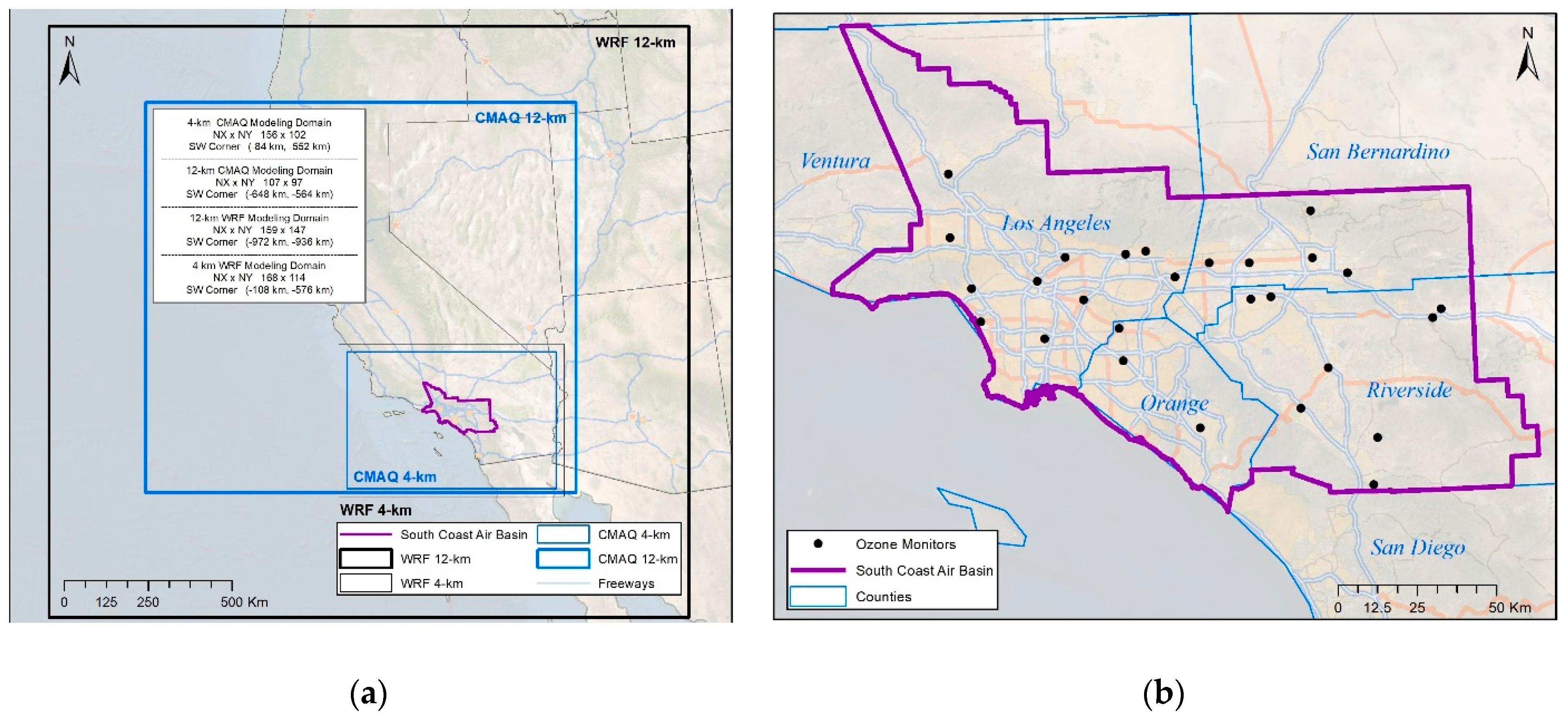
The modeling component of this study was accomplished with the WRF meteorological model and the CMAQ photochemical grid air quality model. The WRF and CMAQ 12-km and 4-km modeling domains are displayed in
Figure 1a, along with the domain parameters.
Figure 1b is a closer look at the SoCAB study region, with ozone monitors indicated and counties labeled. The model projection is Lambert Conic Conformal with latitude of origin = 37.0 N, Central Meridian 120.5 W, and Standard Parallels at 30.0 N and 60.0 N.
2.1. WRF Meteorological Modeling and Model Performance
WRF was used to generate meteorological conditions and inputs for the 4-km and 12-km domains for the mid-May through July period in 2019 and 2020, where mid-May–June 1 is the spin-up period. WRF physics options, performance thresholds, and performance for the 4-km WRF simulations for select surface sites and upper air sites is provided in the
Supplementary Information Document, Section S1. The WRF model performance was typical for a good WRF application. The Meteorology—Chemistry Interface Processor (MCIP) [
21] was used to process the WRF output for CMAQ.
2.2. Emissions Inventories and Processing
Anthropogenic emissions for California were from the ARB 2020 emissions inventory (EI) [
22]. These emissions are available in a “pre-merged” format, which means they are stored by individual source sectors (e.g., on-road, aircraft), which facilitates applying different COVID-19 scaling factors to the different emissions source sectors. Biogenic emissions were based on the Model of Emissions of Gases and Aerosols From Nature (MEGAN) v3.1 biogenic emissions model [
23] with ARB’s adjusted urban leaf area index (LAI) using 12/4-km WRF meteorological data. Fire emissions were based on the Fire INventory from NCAR (FINN) [
24]. Emissions for the Mexico region in the 4 km domain were from the South Coast Air Quality Management Plan (2016 AQMP) EI [
25].
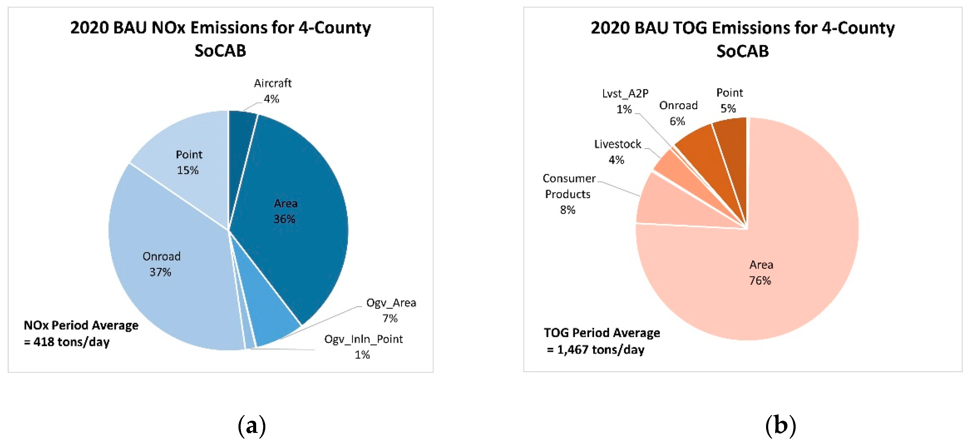
Figure 2 displays the anthropogenic by-sector emissions breakdown for the SoCAB for the ARB 2020 EI. Any sector with less than 1% contribution to the total is not displayed. The period-average is for the period 1 June–31 July 2020.
We developed model-ready emissions for three CMAQ scenarios:
2019 Base Case;
2020 BAU Case;
2020 COVID Case.
The 2019 Base emission were obtained by scaling the ARB 2020 EI. We inspected the 2019 and 2020 California Emissions Projection Analysis Model (CEPAMS) [
26] summertime grown and controlled emissions for the South Coast Air Basin by source sector and found that only on-road was a substantially contributing source (i.e., >3%), with a substantial (i.e., >± 5%) year-to-year change for any pollutant [
26]. Therefore, we kept all sectors besides on-road at the same emissions rate in 2019 as in 2020 and adjusted the on-road sector only. The CEPAM on-road 2019 adjustment factors are as follows: NOx = 1.11, TOG = 1.07, and CO = 1.10. These factors were applied uniformly over the 4-km domain to the on-road emissions for each hour.
2020 BAU emissions were taken directly from the ARB 2020 EI without any scaling adjustment because these emissions we compiled prior to the pandemic and do not account for pandemic effects. The pre-merged categories that comprise this inventory are:
Aircraft;
Area source;
Consumer products;
On-road;
Point (point source format);
Fertilizer;
Livestock;
Lvst (a2p);
Ogv Area;
Ogv Inln (point source format);
Ogv military;
Paved;
Residential Wood Combustion;
Unpaved.
OGV is ocean-going vessels, and Lvst is a second livestock category. Off-road emissions (e.g., construction equipment) are included in the area source category.
2.2.1. 2020 COVID Emissions Adjustments
A bottom-up approach was employed to adjust the 2020 BAU emissions with source sector-specific COVID adjustment factors based on changes in activity. For some sectors, adjustments were developed at a more disaggregated level, namely by Source Classification Codes (SCCs), e.g., within on-road for heavy duty and light duty vehicles, using auxiliary information available within the ARB 2020 EI to determine fractions of subcategories within a sector. Detailed information regarding the data sources utilized, activity basis, geographic and temporal specificity, and derived adjustment factors is provided in the
Supplementary Information Document, Section S3. The sector with the largest NOx reductions is on-road, and the primary data source used to derive the on-road scaling factor was the U.S. Energy Information Administration (EIA) refinery gasoline and diesel sales in California. EIA June and July 2020/2019 fuel sale ratios were 77% for gasoline and 84% for diesel. ARB’s Emission FACtor (EMFAC) tool [
27] was used to calculate Vehicle Miles Traveled (VMT) and appropriately apply scaling factors to the on-road fleet.
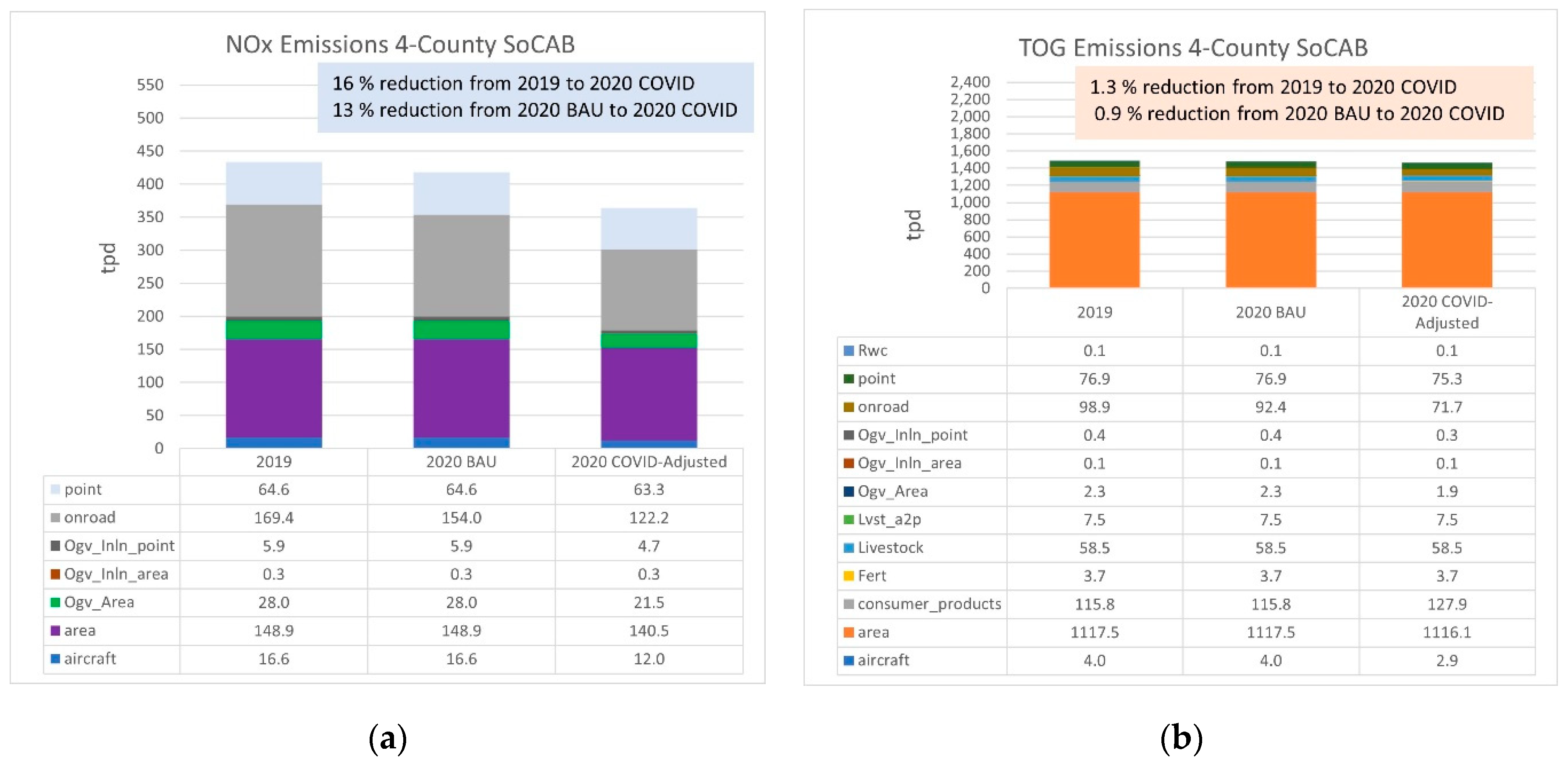
Figure 3 provides a summary of the emissions for the three model scenarios for NOx and TOG in panels (a) and (b), respectively. Note that the TOG emissions adjustments are less than 1% between the three scenarios, because they are dominated by area sources that had a minimal COVID adjustment, and the change in on-road VOC (−27.2 tpd) is partially offset by an increase in the consumer products (+12.1 tpd).
2.2.2. Emissions Processing for Model-Ready Emissions
The 2019 and 2020 adjustment factors were applied to the pre-merged 2020 BAU emissions files.
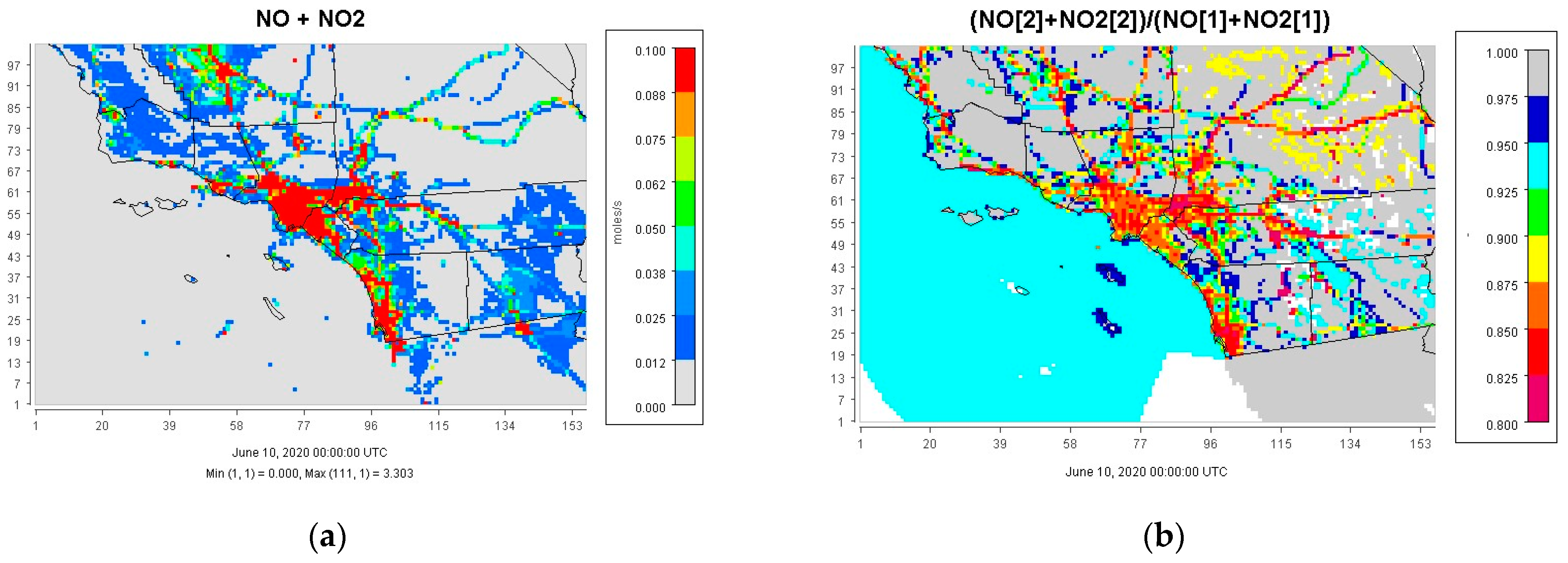
Figure 4 presents examples of the spatial distribution of the merged gridded NOx emissions (NOx ≈ NO + NO
2) for 10 June 2020, at 0:00 UTC in moles/s per 4-km grid cell.
Figure 4a is 2020 BAU and
Figure 4b is the 2020 COVID/2020 BAU ratio (unitless). Note that the conversion factor from moles/s to tons/day for NOx is 4.38.
Figure 4a shows that the highest NOx emissions come from the Los Angeles region as well as along the coast to San Diego.
Figure 4b shows that NOx reductions are approximately 8% over the Pacific due to the OGV reductions and shows a range of reductions throughout the domain and approximately a 10–15% reduction over the SoCAB. For Mexico, the 2020 BAU/2020 COVID ratio is one since those emissions were unadjusted.
2.3. CMAQ Model Configuration
CMAQ version 5.2.1 was run from June through July (with a 10-day spin-up in May) for the 12-km and 4-km modeling domains for 2019 and 2020 for the emissions scenarios previously described. The 12-km simulation results were used solely to derive boundary conditions (BC) for the 4-km simulations. We used the same 2020 12-km BC simulation for both 2020 4-km simulations and the 2019 12-km BC simulation for the 2019 4-km simulation. BCs for the 12-km simulations were from the Whole Atmosphere Community Climate Model (WACCM) [
28], which has 2019 and 2020 model output available, which was utilized for the 2019 and 2020 12-km CMAQ simulations, respectively. Both the 12-km and 4-km simulations used the same science options that are provided in the
Supplementary Information Document, Section S2. The model was run on a multi-processor machine with 24 processors (6 NCOLS × 4 NROWS).
2.4. CMAQ Operational Model Performance Evaluation
The AMET tool was used to evaluate the CMAQ simulations using concurrent ozone observations. Model performance statistics (i.e., bias, error, and correlation) and time series plots were calculated at monitoring sites. Scatter plots of predicted and observed concentrations were generated as well as spatial maps of site-specific performance statistics. Emery et al. [
29] provide a set of statistics and benchmarks to assess PGM performance. They deemed that normalized mean bias (NMB) and error (NME) and correlation (r or COR) statistics have the best characteristics historically.
Table 1 presents the statistical measures and goal and criteria thresholds for ozone for NMB, NME, and COR. Goal thresholds represent the statistical values that approximately one-third (i.e., the 33rd percentile) of top performing past applications have achieved and are considered the best a model can be expected to achieve. The less restrictive criteria are around the 67th percentile and indicate statistical values that approximately two-thirds of past applications have met. Additional relevant recommendations include: (1) no minimum cutoff for maximum daily 8-h average (MDA8) ozone; (2) temporal scales for ozone statistics should not exceed 1 month; and (3) spatial scales should range from urban to ≤1000 km.
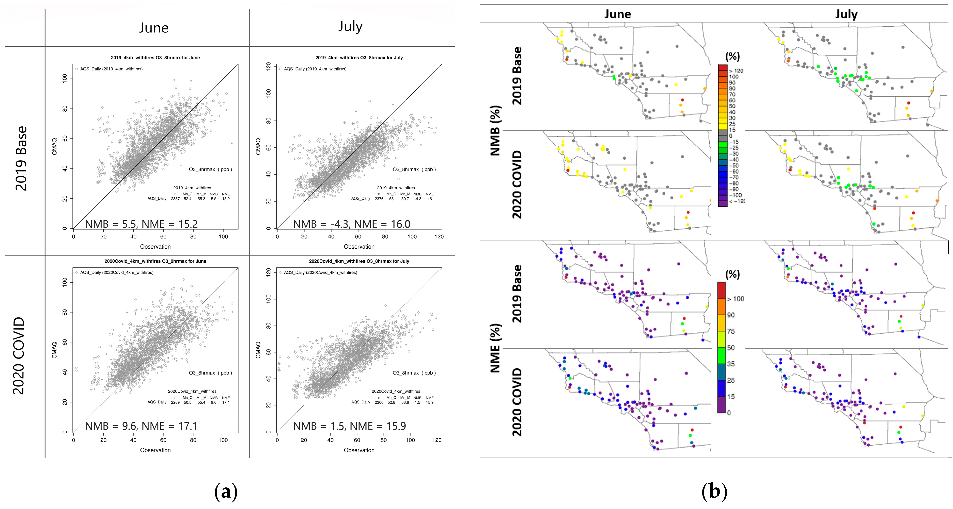
Figure 5a shows scatter plots of MDA8 ozone performance for all sites in the 4-km domain for June and July for 2019 and 2020 COVID. The
x-axis is observed MDA8 ozone, and the
y-axis is CMAQ MDA8 ozone. Each point represents MDA8 ozone for one site on one day. NMB and NME are displayed in
Figure 5a. For each case, the NME is between 15.9% to 17.1%, which easily meets the performance criterion and nearly meets the criteria goal. NMB has more variation between the four cases. For 2019, there is a positive NMB of 5.5% in June and a negative bias of −4.3% in July; these values are close to the performance goal. For 2020, there is a positive NMB of 9.6% in June and 1.5% in July. For both years, July exhibits a discernable negative bias at the higher range of observed MDA8 (e.g., >80 ppb).
Figure 5b presents spatial plots of site-specific NMB and NME statistical performance metrics for 2019 Base and 2020 COVID. For June, the majority of SoCAB monitors meet the NMB criteria, and all sites meet the NME criteria in both 2019 and 2020. For July, there is an underestimation bias at many monitors in the SoCAB in both 2019 and 2020, but the NME falls within the criteria. Outside of the SoCAB, CMAQ tends to overestimate ozone for both months and both years at some sites.
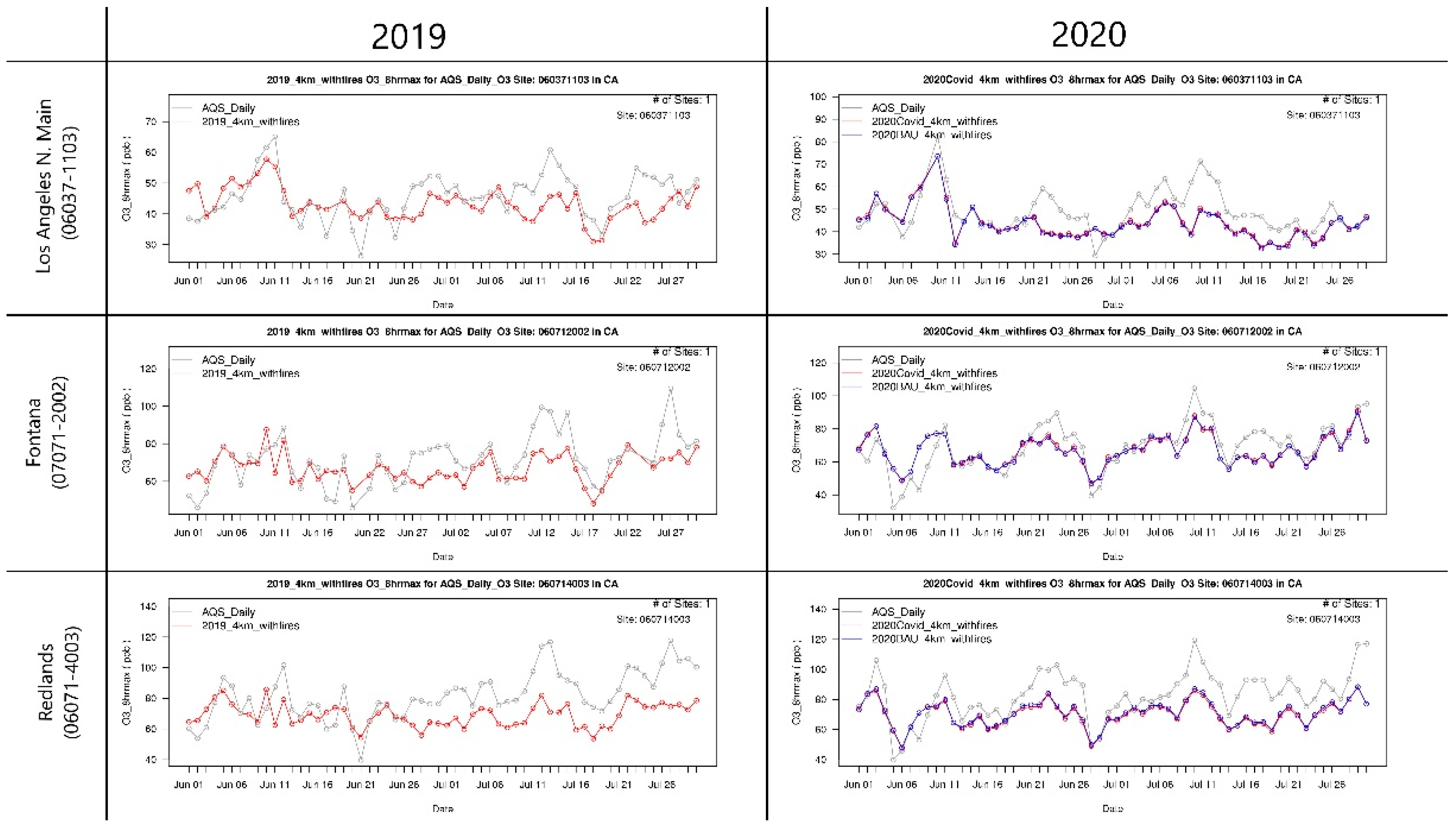
The
SI (Section S4) presents additional performance statistic on a per monitor basis, including timeseries plots and statistics tables for ten selected sites that span the SoCAB. As an example, three timeseries plots are shown in
Figure 6 (the location of these three sites can be found in a later section). Note that differences between the 2020 COVID and 2020 BAU timeseries plots shown in the right panels of
Figure 6 are small and overshadowed by day-to-day variations; these small differences are consistent with the spatial plot results shown later. The statistics tables in
SI Section S4 and the time series plots show that, for both 2019 and 2020, NMB performance is superior in June (most sites meet the NMB goal) compared to July (negative bias at all but one site and many sites do not meet the criteria). Investigating why the July performance is inferior to June was beyond the scope of this study, but we note that the period-wide highest days are mostly in July and the CMAQ model does not fully capture the highest days. A similar phenomenon is observed in the SCAQMD 2016 AQMP [
25] performance for the “Urban Receptor” monitors that correspond to the San Bernardino monitors, where the negative bias is more severe in July than in June. Overall, ozone model performance was generally within typical thresholds based on historical PGM applications.
We do not present a NOx model performance analysis because the operational AMET products for nitrogen species may fail to give meaningful results because most commercial NOx analyzers do not measure true NO
x. Instead, they measure NOγ where NOγ = NO
x + nitrous acid (HONO) + nitric acid (HNO
3) + others nitrogen species; therefore, as Dickerson et al. [
30] point out, standard NOx evaluations may involve errors of a factor of two or more. There are approaches to reduce the impact of the interfering species by focusing on early morning hours when the NOx species are expected to dominate the NOγ, as per Toro et al. [
31], which we recommend for future work.
We performed a fire emissions sensitivity test for the 2020 COVID case by eliminating fire emissions (i.e., we performed a “zero-out” simulation) and found that during the June–July 2020 period fire impacts on ozone concentrations were negligible.
2.5. Evaluation Approach
Recall that this study had two main goals: (1) to perform a dynamic model evaluation of the CMAQ model to determine whether it can reproduce the observed ozone response due to the sudden emissions reductions associated with the COVID-19 pandemic; and (2) to examine the impacts of the COVID-19 emissions reductions in the SoCAB with CMAQ. The first goal is accomplished by considering the two scenarios that occurred (i.e., 2019 Base and 2020 COVID) and comparing the modeled responses and observed ozone responses. The second goal is accomplished by comparing the two 2020 modeled scenarios (i.e., 2020 COVID and 2020 BAU).
2.5.1. Dynamic Evaluation Methodology
For the dynamic evaluation, we follow the EPA modeling guidance procedures [
14] for projecting ozone concentrations in an ozone model attainment demonstration. This approach was used in the SCAQMD’s AQMP [
25] to define ozone attainment VOC/NOx emission control strategies. The 2020 COVID Case represents the future-year emissions scenario, and 2019 Base Case represents the base year. Typically, the future year for a model attainment demonstration may be five or more years in the future (or a decade or more for the SoCAB extreme ozone NAA), but the abrupt emissions reductions due to COVID-19 restrictions mimic a potential future-year scenario and has the unique attribute of having observations for the comparison. In a typical model attainment demonstration, the meteorology is the same for the future and base years because the future-year meteorology is unknown. For this analysis, however, the meteorology is different between 2019 and 2020, although the June–July 2019 and 2020 modeling periods were selected to have similar meteorology. The EPA recommends using model estimates in a relative rather than absolute sense to reduce potential model bias effects for making future-year ozone projections. Fractional changes in air pollutant concentrations between the model future-year and model-base-year are calculated; these ratios are called relative response factors (RRFs). The RRFs are multiplied by base-year-observed ozone concentrations to predict future-year ozone concentrations. The base-year observations are the average of three-years of design values (DVB; defined below), and the future-year ozone design value (DVF) projection formula is as follows:
where DVF
i is the estimated design value for the future year in which attainment is required at monitoring site i; RRF
i is the relative response factor at monitoring site i; and DVB
i is the base design value at monitoring site i.
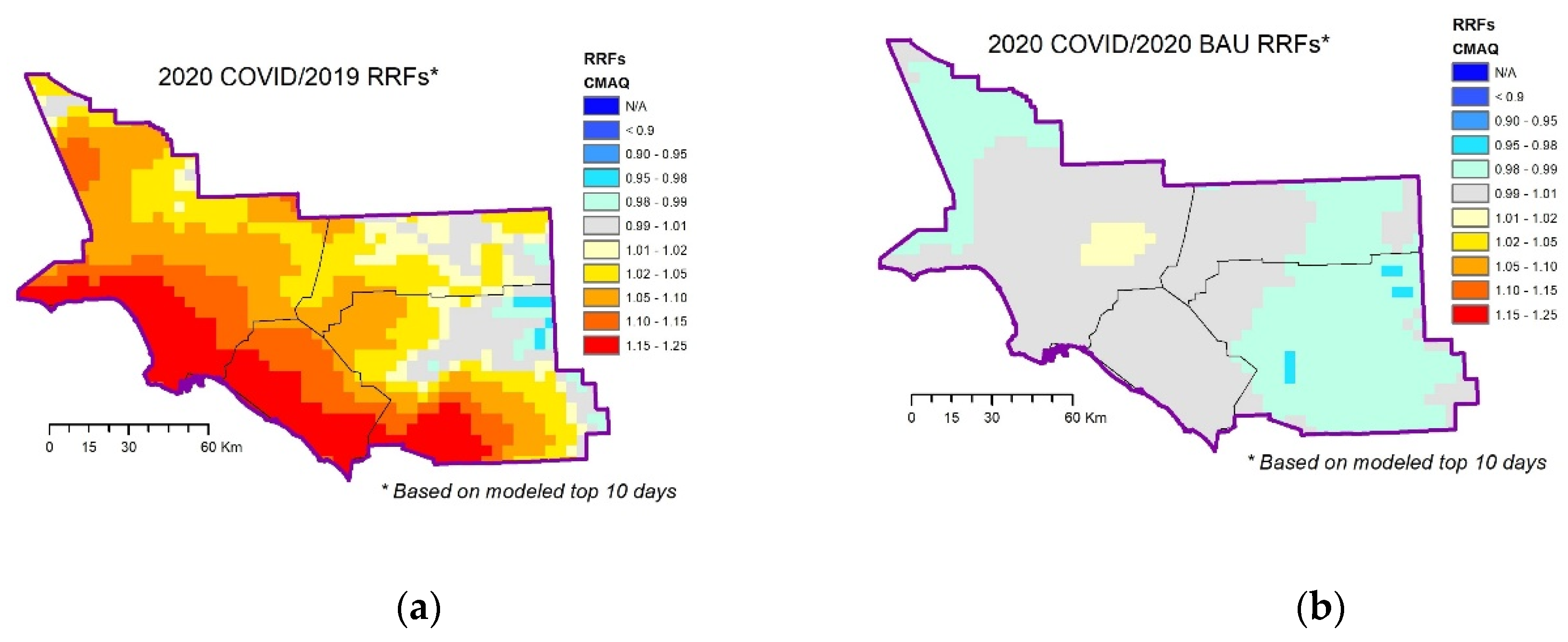
We calculate RRFs as one would do for projecting future-year ozone design values, only instead of using modeling results for a base- and future-year emissions scenario with the same meteorological inputs, we use the modeling results for the 2019 Base Case and 2020 COVID Case that have different meteorology. We also calculate observation-based RRFs using the 2019 and 2020 ozone observations in a consistent fashion. We do not use the design values in our analysis because we only model 2 months, which is not long enough to define design values, therefore we only focus on the RRFs.
There are additional considerations for the RRF calculations regarding which days to use in the RRF calculation, and EPA guidance has evolved over the years. We follow the current EPA recommendation, which is to calculate RRFs based on the 10 highest modeled days in the base year. This is to reflect the fact that design values are based on the three-year average 4th high observed MDA8 ozone values. The EPA recommends “
selecting a set of modeled days that are likely to encompass a range of values that are somewhat higher than and somewhat lower than the 4th high value… this balances the desire to have enough days in the RRF to generate a robust calculation, but not so many days that the RRF does not represent days with concentrations near the observed design values” [
14]. We follow EPA recommendations to evaluate CMAQ using the standard regulatory procedures so that the results are relevant to the regulatory community. The EPA describes an additional basis for their guidance and reports that “
model response to decreasing emissions is generally most stable when the base ozone predictions are highest. The greater model response at higher concentrations is likely due to more “controllable” ozone at higher concentrations… In most urban areas, on days with high ozone concentrations, there is a relatively high percentage of locally generated ozone compared to days with low base case concentrations. Days with low ozone concentrations are more likely to have a high percentage of ozone due to background and boundary conditions.” There are additional EPA specifications regarding the MDA8 ozone value (i.e., ≥60 ppb) and the number of days that meet that criterion. In our analysis, that criterion is generally met, but for monitors that do not meet the minimum number of days ≥ 60 ppb threshold, we proceed with the analysis with MDA8 < 60 ppb. In addition, we use a single-grid cell rather than the 3 × 3 array recommended by the EPA. Our procedure is as follows:
For 2019 Base and 2020 COVID, identify the top 10 (T10) modeled days for MDA8 ozone and calculate the average of those days;
For 2019 and 2020, calculate the average observed MDA8 ozone on the T10 modeled days;
Calculate RRFs as the ratio of 2020 COVID to 2019 Base for modeled T10 MDA8 ozone and observed T10 MDA8 ozone.
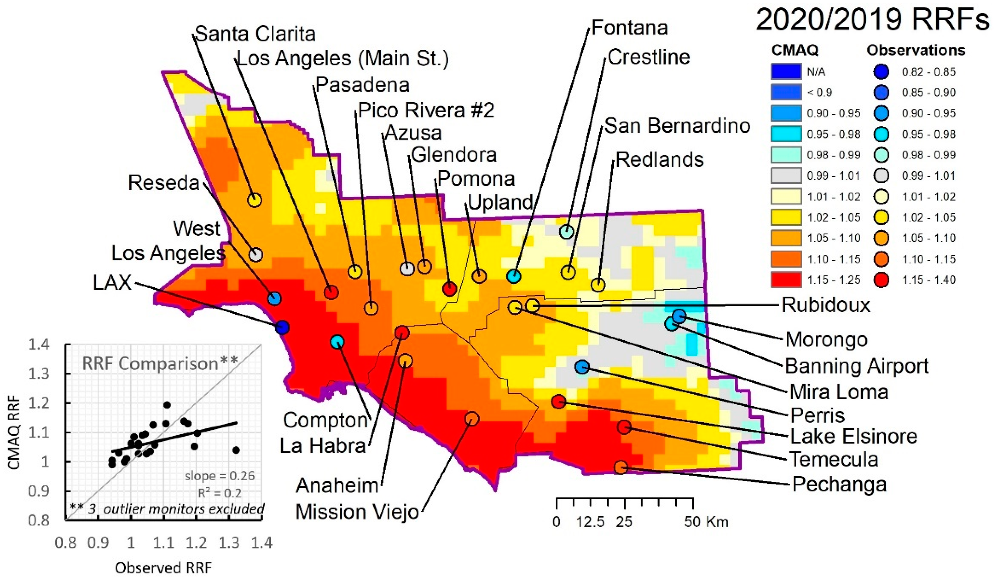
We do this for each SoCAB grid cell that contains a monitor to obtain a modeled/observed pair of RRFs at each monitoring site. In addition, for all model grid cells we calculate T10 modeled RRFs over all the SoCAB grid cells. In general, the T10 days may be different at each grid cell.
2.5.2. T10 Days Standard MPE
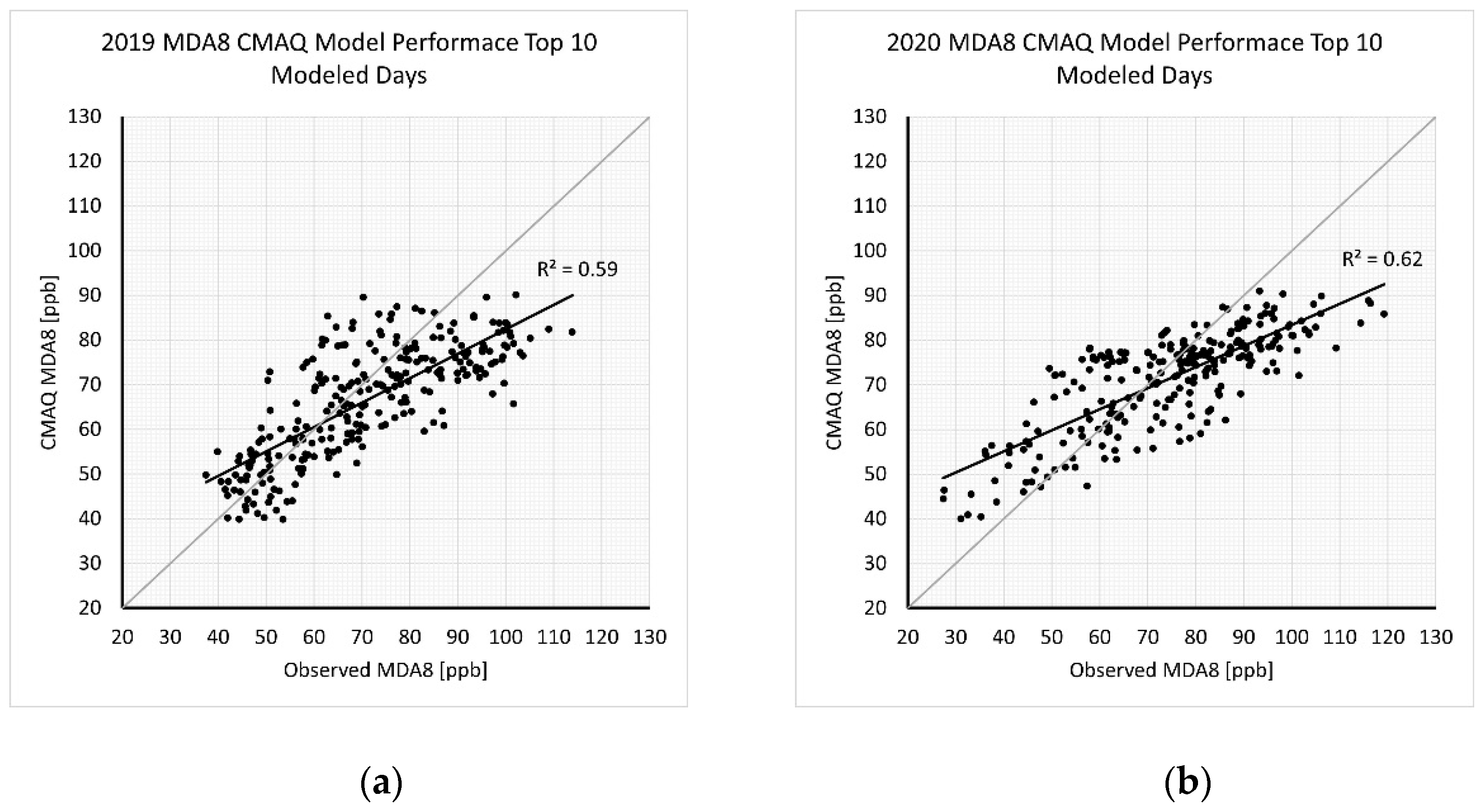
Prior to the dynamic model performance evaluation, we examined the model performance for the T10 modeled days that are used to calculate the RRFs.
Figure 7 presents a scatter plot of observed versus modeled MDA8 for each day in the T10 modeled days at each monitoring site for 2019 and 2020 in panel (a) and (b), respectively. These points are a subset of the data in
Figure 5a. Considered across all sites, the model performance is similar between the two years and has a similar underestimation bias that almost achieves (−6.3% in 2019) or does achieve (−4.0% in 2020) the ozone performance goal for NMB (±5%), with NME achieving the performance goal in both years (<15%). However, the model underestimates the highest observed MDA8 ozone concentrations. Model performance statistics for the selected sites is shown in
Table 2.
4. Discussion
The dynamic model evaluation component of this study showed that, throughout much of the SoCAB, CMAQ can replicate the observed ozone response to the COVID-19 emissions reductions and changes in meteorology between 2019 and 2020 using the EPA’s ozone projection procedures. The modeled ozone response was, however, generally weaker than observations. This is similar to the finding of Karamchandani et al. [
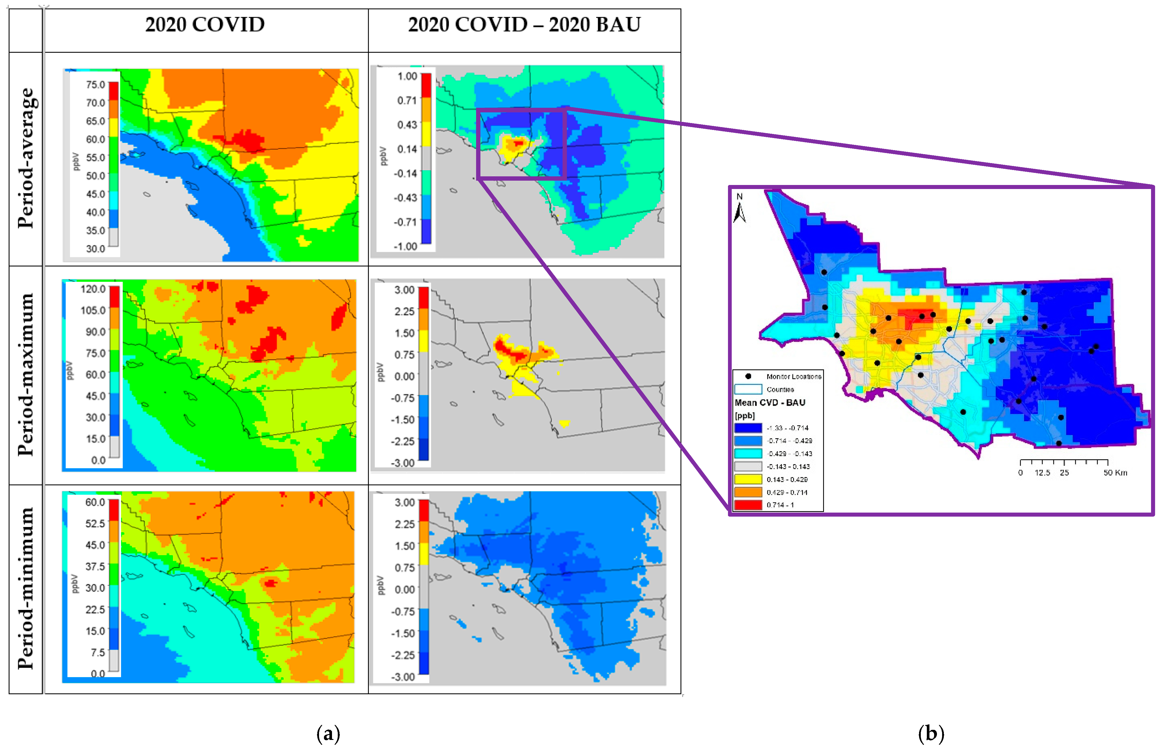
15], who found the CMAQ model to be “stiff” (i.e., underpredicted the ozone response). Our results of the evaluation of the COVID-19 impacts with CMAQ showed variable ozone response to NOx reductions across the SoCAB, with an approximately 50 km × 50 km region in Los Angeles County that had average MDA8 ozone increases, and elsewhere throughout the SoCAB there were ozone decreases. This result agrees with regional modeling studies that use different air quality models and grid resolutions (e.g., Campbell et al. [
6], Gaubert et al. [
7], and Keller et al. [
8]), which found similar variable ozone responses with localized increases in urban areas. This suggests that this phenomenon is robust to different air quality models at differing spatial scales.
This study is limited by a few factors: (1) relatively small COVID-19 emissions reductions (i.e., ~13% NOx); (2) limited spatial and temporal resolution for the emissions adjustments (i.e., no day-of-the-week effect for on-road adjustments); (3) non-COVID adjusted boundary conditions (COVID adjusted boundary conditions would account for regional and global background changes in ozone and ozone precursors transported into the SoCAB via boundary conditions); and (4) uncertainties in emissions, in particular, VOCs and biogenics. Regarding the third limitation, Bouarar et al. [
32] investigated the response of chemical species in the free troposphere during the COVID-19 pandemic using the CAM-chem model and found zonally averaged ozone to be 5–15% lower than 19-year climatological values. Their modeling successfully reproduced the observed ozone anomalies during the 6 months that followed the COVID-19 outbreak that were presented in Steinbrecht et al. [
33]. The 2020 anomaly compared to climatology was found to be primarily due to reduced air traffic, reduced surface emissions, and anomalous 2020 meteorology. It is unclear how potential longer-term trends were considered and accounted for over the climatological period. Our future work will consider the impact of COVID-19 effects on free tropospheric ozone and transport from outside the SoCAB. Omission of a potential reduction in background ozone may plausibly contribute to the CMAQ model “stiffness” described above, but due to the non-linearity of ozone formation and because the SoCAB encompasses both VOC and NOx-sensitive regimes it is difficult to predict how the model would respond to combined changes (i.e., background ozone plus local emissions reductions) across the SoCAB; however, we note that our findings could change substantially under that scenario. Typically for model attainment demonstrations, such as the SCQMD 2016 AQMP [
25], global BCs are held constant due to lack of accurate information to make an adjustment, and the analysis in this study is consistent with that approach. If future work shows substantial differences in modeled ozone responses due to background ozone, the effects of background ozone on model attainment demonstrations should be explored.
Recommendations for further study are as follows:
Obtain, evaluate, and utilize WACCM 2020 COVID impacted BCs for the 2020 COVID simulation. This will provide a more complete assessment of the COVID impacts and enable a comparison of the effect of local versus background COVID impacts;
A targeted NOx model evaluation and VOC evaluation;
A more rigorous WRF evaluation including an assessment of the marine layer;
Day-of-the-week adjustment to the on-road sector to allow for day-of-the-week analyses to provide additional insight into the current extent of VOC-limited versus NOx-limited chemical regimes.


