

The Spatial Data Analysis of Determinants of U.S. Presidential Voting Results in the Rustbelt States during the COVID-19 Pandemic

Department of International Business, Chung Yuan Christian University, No. 200 Zhongbei Rd., Zhongli District, Taoyuan City 320314, Taiwan
ISPRS Int. J. Geo-Inf. 2023, 12(6), 212; https://doi.org/10.3390/ijgi12060212
Submission received: 4 February 2023
/
Revised: 12 May 2023
/
Accepted: 19 May 2023
/
Published: 23 May 2023
(This article belongs to the Special Issue Human-Induced Disaster and Conflict Analysis, Prediction, and Prevention by Geospatial Analytics and Information Systems)
Abstract
:This study aims to analyze the factors that determine voting behavior in the rustbelt states during the 2020 U.S. presidential election. The rustbelt states are traditionally considered “swing states” and play a crucial role in determining the outcome of the presidential election. The study employs a spatial econometrics model that considers COVID-19-related factors, such as the percentage of people wearing masks and the number of COVID-19 deaths in each county of the rustbelt states. Firstly, the study identifies the most suitable spatial econometrics model. Secondly, the study shows that COVID-19 pandemic-related independent variables had a significant positive impact on the Republican Party’s results in the U.S. presidential election while mask-wearing behavior had a significant negative impact. These results suggest that the COVID-19 pandemic has influenced voting behavior and altered the political landscape, but it does not have geographical effects.
1. Introduction
The 2020 U.S. presidential election was impacted by the consequences of the COVID-19 pandemic. The existing literature suggests that the fear generated by the pandemic may have increased political polarization [1,2]. During natural or human-made disasters, some people tend to seek comfort by supporting conservative political views and the ruling party, while others may opt to vote for the opposition party as a way to punish poorly managed political leaders. Since the measures taken during the COVID-19 pandemic were implemented hastily and without thorough public deliberation, it is possible that this could have further fueled public dissatisfaction [3]. Previous studies indicate that people tended to initially support their governments during the early stages of the pandemic [4]. However, political polarization can affect how policies related to the COVID-19 pandemic are evaluated. Some voters may cast their vote for the opposition party due to the severity of the pandemic, while others may base their decision on the political leaders’ response to the situation [5].
The previous literature on the 2020 U.S. presidential election has primarily focused on the impact of COVID-19 on the Republican Party’s support rate and the election results. Hart suggests that the pandemic reduced support for Donald Trump but increased support for independent voters [6]. Baccini et al. also found that COVID-19 cases had a negative effect on Trump’s re-election campaign, particularly in urban areas [7]. They also suggest that the pandemic had a positive effect on voter mobilization for Joe Biden.
The rustbelt states, which include Illinois, Wisconsin, Indiana, Michigan, Ohio, West Virginia, Pennsylvania, and New York State, have traditionally been critical “swing states” in presidential elections (https://beltmag.com/mapping-rust-belt/ (accessed on 2 February 2023)). However, in the past five years, there has been an increase in geographical and racial differences among the counties in these states, leading to more politically polarized conditions [8,9]. The results in the rustbelt states have a significant impact on the overall outcome of the U.S. presidential election, yet there has been a lack of analysis on the voting results in these states. Gimpel found that some counties in the rustbelt states switched their support to the Democratic Party in the 2020 presidential election [10]. Therefore, it is important to examine the factors which influence voting results.
In light of this, our study aims to analyze the effects of the COVID-19 pandemic, as well as the influence of geographical and economic variables, on the Republican Party’s support rate in the 2020 U.S. presidential election in the rustbelt states.
The structure of this research study was as follows: The Research Method indicated our research design and related descriptive statistics of the dependent and independent variables. The Discussion stated the results of the research model. The research findings were listed in the Conclusions section.
2. Research Methods
2.1. Research Questions
The study aimed to investigate the impact of COVID-19-related factors on the U.S. presidential election results, specifically in the rustbelt states where prior literature studies have not explored this topic. The researchers sought to identify relevant COVID-19 pandemic-related factors and economic variables to build spatial econometrics models.
During the pandemic, mask-wearing is critical to public health to mitigate the spread of the virus. However, in the U.S., the issue of mask-wearing has become politicized. President Trump initially opposed the CDC’s recommendation to wear masks, creating a political divide. As of August 2020, 16 states with Republican governors did not have mask regulations, unlike 34 other states and Washington D.C. Prior research has also shown a negative correlation between mask-wearing behavior and support for Donald Trump in the 2016 presidential election [11]. Therefore, the study includes mask-wearing behavior as one of the COVID-19-related independent variables and raises the research question of whether mask mandates are related to the 2020 U.S. presidential election results in rustbelt states.
During the COVID-19 outbreak, the fatality rate among people over 65 years old was higher compared to other age groups, as per CDC data in the U.S. Given that older individuals tend to vote more frequently than other age groups and make up a significant portion of all U.S. voters, the higher fatality rate during the initial stages of the COVID-19 pandemic in 2020 may have resulted in a potential shift in the presidential election results. Therefore, the study aims to investigate whether the death toll from the COVID-19 pandemic impacted the U.S. presidential election results in rustbelt states. This forms the basis of the second research question.
The study also incorporates control variables such as housing units (in each county), education, household income, and unemployment rate in constructing the spatial econometrics model.
In U.S. census data, housing units refer to a house, apartment, mobile home, or any other structure that is used as a place of residence by one or more persons. It is the basic unit of measure for housing in census data and is used to provide information on the number of housing units, their characteristics, and the people living in them. Housing units are classified as either occupied or vacant and may be owned or rented by the occupants. Housing unit data are important for understanding the housing market, population demographics, and community development. For education data, this study chose the number of high school graduates or above in each county. It is because the selection of education data considers the actual condition in the demographic characteristics of the U.S. The unemployment rate and household income in each county are common representative economic variables in related research.
Therefore, the third research question aims to explore whether the U.S. presidential election results were influenced by the number of housing units, voter education level, household income, and unemployment rate in each county.
2.2. Data Description
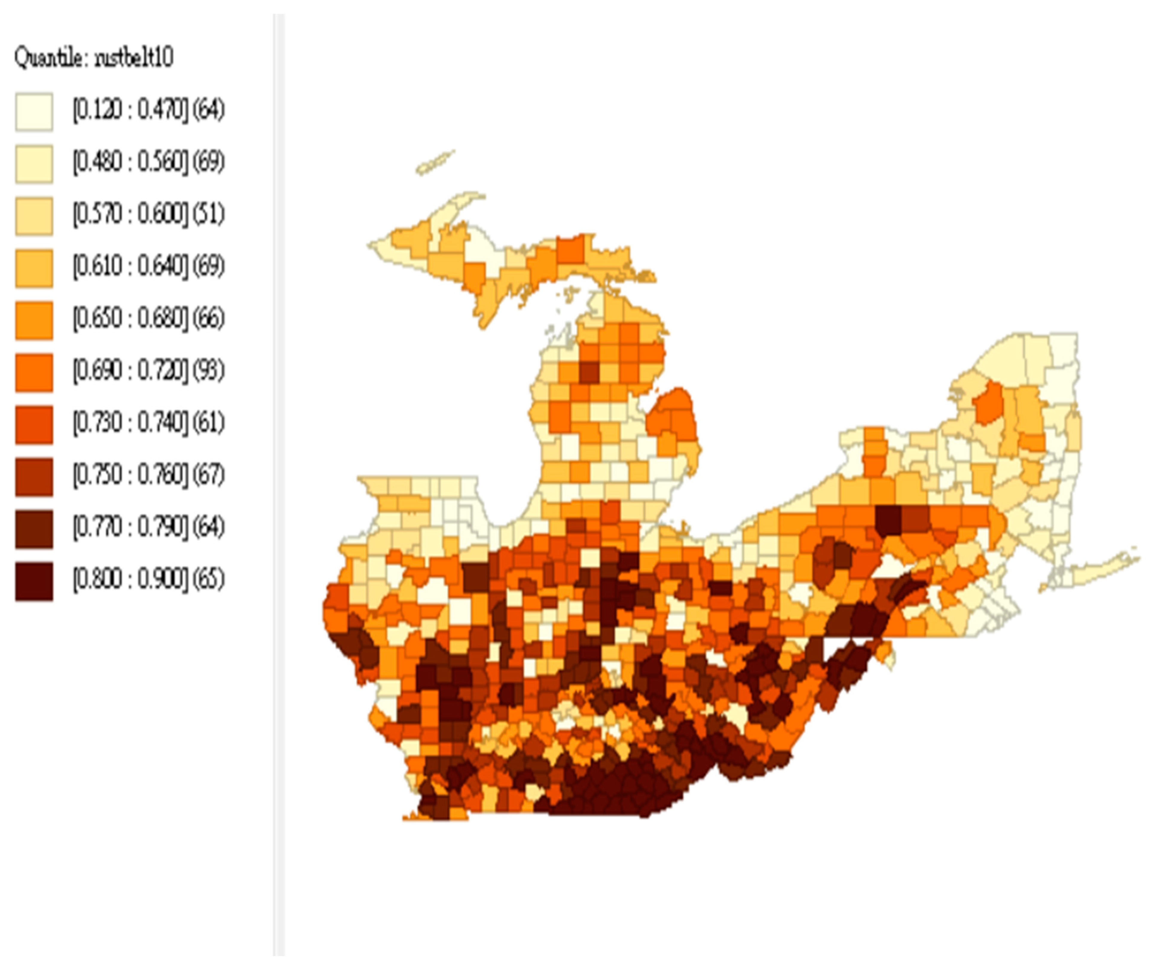
The purpose of the study was to investigate the impact of the COVID-19 pandemic on the 2020 U.S. presidential election. In order to achieve this, this study used the results of the 2020 U.S. presidential election as the dependent variable. Based on the findings presented in Figure 1, it was observed that the Republican Party received a greater share of the votes in the southern rustbelt states, including Indiana, Ohio, and West Virginia. This information was used as the dependent variable (Y) in this study.
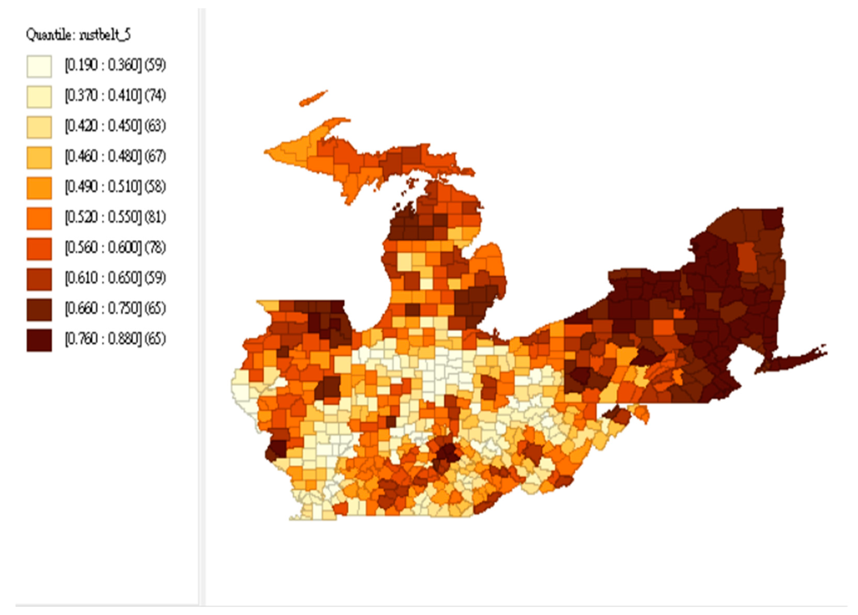
To assess mask-wearing behavior, this study utilized data collected by Dynata, a survey firm. Between 2 July and 14 July 2020, Dynata conducted a survey of 250,000 respondents. The survey asked whether respondents frequently wore face masks in public, offering response options of “always”, “frequently”, “sometimes”, “rarely”, and “never”. Figure 2 illustrates the proportion of respondents who reported that they often wore face masks. We utilized these mask-wearing data from July 2020 since the timing of the survey coincided with the U.S. presidential election, making it of particular relevance and value as a reference point.
In comparison to Figure 1 and Figure 2, our analysis revealed that the eastern rustbelt states had a higher proportion of respondents who reported frequently wearing masks while also being regions where Republicans received fewer votes in the 2020 presidential election.
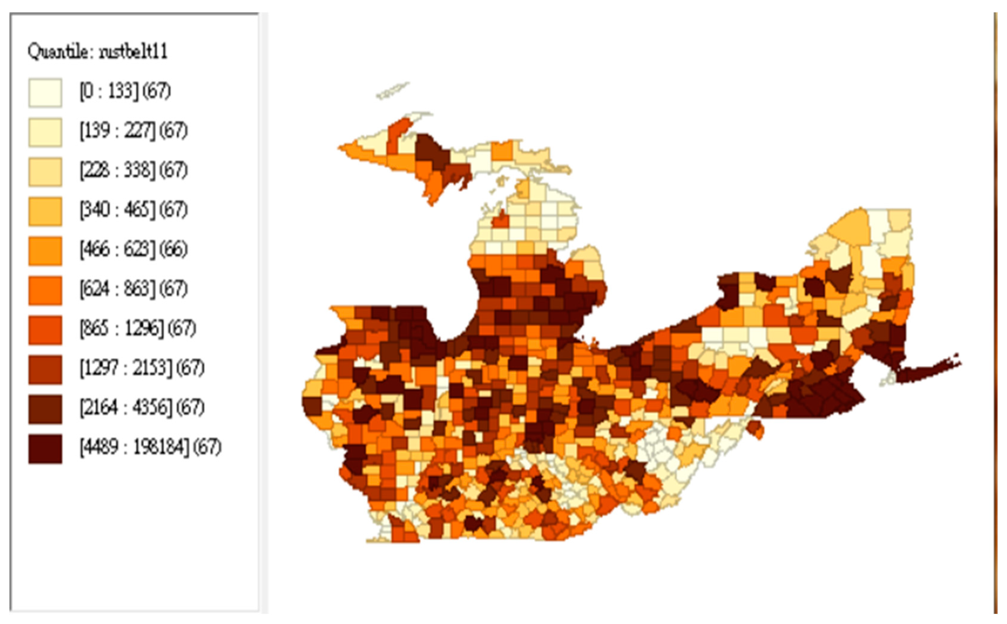
Furthermore, our study investigated the relationship between the COVID-19 pandemic and the U.S. presidential election by examining the total number of COVID-19 cases and the death toll prior to the election. Figure 3 depicts the total number of COVID-19 cases prior to the election.
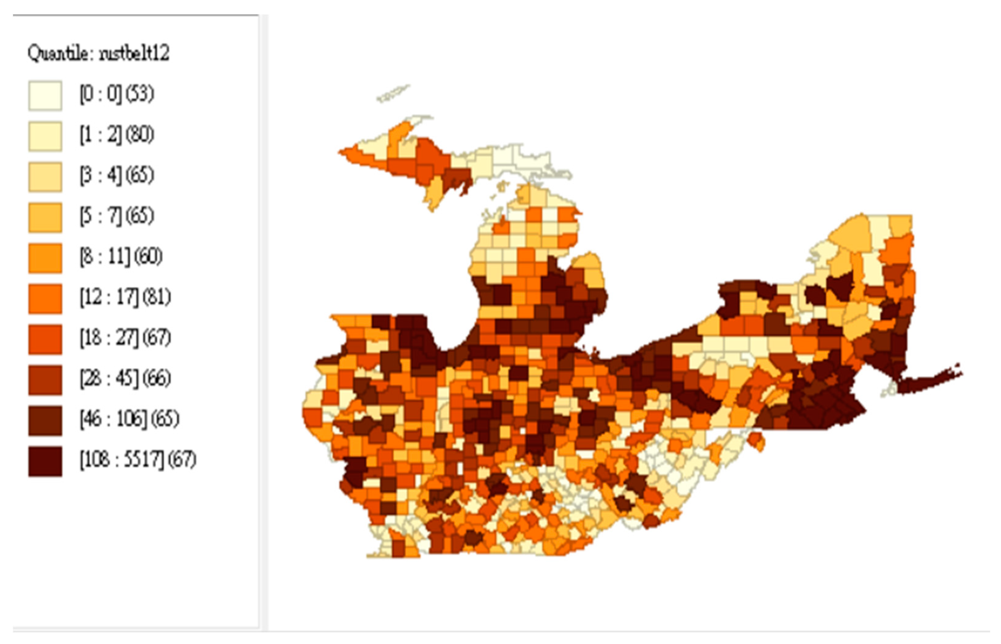
Figure 4 displays the total number of deaths from COVID-19 prior to the U.S. presidential election. Our analysis suggests a correlation between the percentage of Republican votes, the percentage of individuals wearing masks, and the number of deaths due to the virus.
In the subsequent section of our study, we will employ a spatial econometrics model to evaluate the significance of the public health variables in our model.
This study selected six independent variables to examine the factors that may have influenced the U.S. presidential election results. The six independent variables, dependent variable, and descriptive statistics are listed in Table 1 and Table 2.
In order to avoid the influence of the large discrepancy among variables on the spatial regression models, we make all of the variables standardized.
2.3. Spatial Regression Model
This study utilized the spatial cross-sectional regression model to evaluate the influence of regional factors, COVID-19 pandemic-related factors, and economic factors on the voting results for Donald Trump in the 2020 U.S. presidential election.
A spatial cross-sectional regression model is a type of spatial econometric model used to analyze data that is both cross-sectional (i.e., collected at a single point in time) and spatially dependent (i.e., influenced by the values of neighboring observations).
In this model, the dependent variable is regressed against both independent variables and spatial lag variables, which account for the impact of neighboring observations on the dependent variable. The independent variables are chosen based on their relevance to the research question and ability to explain variation in the dependent variable.
The model also takes into account spatial autocorrelation, which occurs when the values of a variable in one location are correlated with the values of the same variable in nearby locations. This is performed by incorporating a spatial weight matrix, which assigns weights to the neighboring observations based on their proximity to the observation being analyzed.
Overall, the spatial cross-sectional regression model is a useful tool for analyzing spatially dependent cross-sectional data, allowing researchers to account for the effects of both independent variables and spatial dependencies when modeling the relationship between the dependent variable and its predictors.
This study followed the spatial econometrics theory to select a suitable model. For the spatial cross-sectional data, we began with the linear spatial regression model.
The study used the following spatial linear regression models to construct the spatial cross-sectional regression models according to the previous literature [12].
- (1)
- General Nesting Spatial (GNS) model: The model’s general form is listed below:
In Equation (1), is the spatially lagged dependent variable, is the lagged explanatory variable, is the spatial lag of disturbance terms, and wij is the N × N spatial connectivity matrix.
- (2)
- SARAR (SAC) model: In Equation (1), we assume γ = 0. The general form is listed below:
This model includes a spatially lagged dependent variable and a spatially autocorrelated error term.
- (3)
- Spatial Durbin model: The model contains the independent variables, spatially lagged dependent variables, and spatial lag of the covariates. The general form is shown below:
- (4)
- Spatial Durbin Error Model: The model assumes that ρ Equation (1) equals 0. The general form is in Equation (4)
- (5)
- Spatial lag model: The model assumes there are interactions in the dependent variable. The general form is in Equation (5):
- (6)
- Spatial error model: The model assumes there are interactions in the disturbance term. The general form is in Equation (6):
2.4. Spatial Matrix
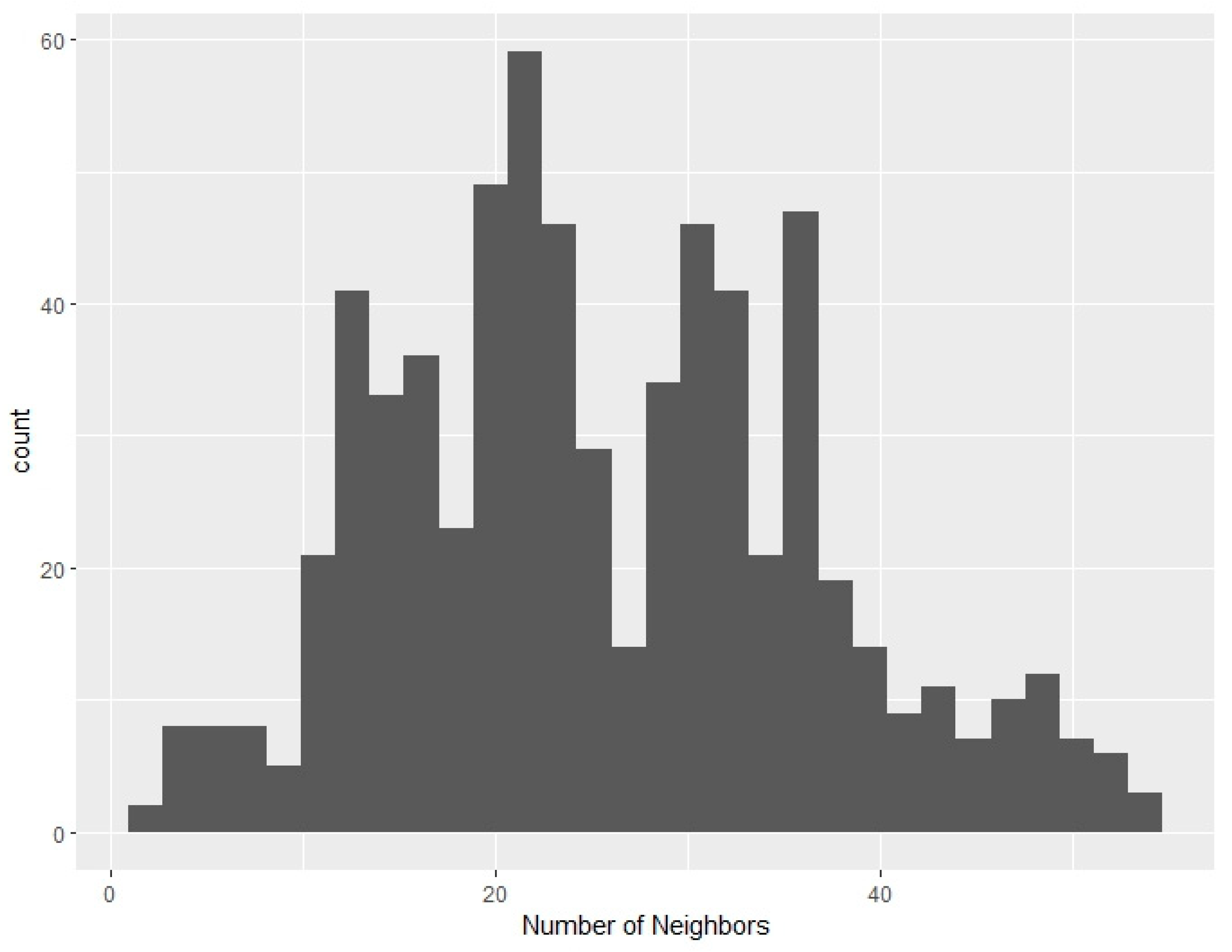
This study constructed the spatial matrix according to a matrix of the k nearest neighbors (knn). The k nearest neighbors (knn) matrix is commonly used for analyzing point data as it only considers points and not areas. However, an area’s knn matrix can be created by first determining its centroid (center of gravity) and analyzing the points instead. For point data, the number of neighbors is usually determined through modeling or experience, but for area data, the neighborhood structure depends on the shape and surface of the regions designated by the centroids. The distance between centroids can cause a narrow and long region not to be one of the closest neighbors, even though it meets the contiguity criterion [13]. The simplest way to create a spatial weights matrix based on distance is to consider two points i and j as neighbors if j is within a certain distance from i. Specifically, wij = 1 if the distance between i and j (dij) is less than or equal to a predetermined cutoff value (δ), and wij = 0 if it is greater than δ.
This study constructed the spatial matrix by the “spdep” function of the R language. The spatial weighted matrix was composed of 0 and 1 with standardized rows. The distribution of the neighbor graph is shown in Figure 5.
3. Results
3.1. Model Selection
The study used the R language to conduct all related spatial regression analyses and the Geoda software to construct all the figures shown in the previous section. In order to create a suitable spatial regression model, this study considers using the k-nearest neighbor matrix by setting k = 2. The matrix guarantees a set number of adjacent areas for each region under consideration, making it particularly valuable in handling an uneven patchwork.
This study used the library of “spdep” and “spatialreg” of the R language to construct the spatial cross-sectional regression model [14,15]. We constructed the spatial regression models from the most general spatial specification, including the above-mentioned six models. In the beginning, we used the COVID-19 cases in each county (cases) as the independent variable that represents the COVID-19-related variable. After we constructed the six related spatial regression models, we used the AIC value as the standard to choose the suitable model. The model with the lowest AIC value is the most suitable model. Table 3 is the AIC values of the six spatial regression models. The coefficients of all models in which COVID-19 cases as the independent varia-ble are listed in Table A1. In addition, the coefficients of all models in which COVID-19 deaths as the independent variable are listed in Table A2.
The study found the AIC value of the Spatial Durbin model had the lowest AIC value. Therefore, we chose the Spatial Durbin model as our final model. The results of the Spatial Durbin Model were shown as Table 4:
According to the results, we also found that ρ (rho) was 0.338, the LR test value was 77.132, and the p-value < 0.0001. It indicated a strong spatial autocorrelation in the dependent variable. This study also made the LM test for residual autocorrelation; the test value was 0.687, and the p-value was 0.407 > 0.05. It showed that the null hypothesis of no residual autocorrelation is not rejected, and it was concluded that the model adequately accounts for the spatial dependence structure in these data. This study made the test in order to know whether the SDM model degenerated to the SEM model [16]. We found the Likelihood ratio = 61.821, p-value < 0.0001. It rejected the null hypothesis, and λβ + γ ≠ 0 (λ, β, and γ are the coefficients in Equations (3) and (6). The Spatial Durbin Model still holds.
The study also used the COVID-19 death cases in each county (deaths) as the independent variable, which represented the COVID-19-related variable. We also used the AIC value to choose the most suitable model. Table 5 is the AIC values of the six spatial regression models.
The study found the AIC value of the Spatial Durbin model had the lowest AIC value. Therefore, we chose the Spatial Durbin model as our final model. The results of the Spatial Durbin Model were shown as Table 6:
According to the results, we also found that ρ (rho) was 0.337, the LR test value was 76.784, and the p-value < 0.0001. It indicated a strong spatial autocorrelation in the dependent variable. The study made the LM test for residual autocorrelation; the test value was 0.627, and the p-value was 0.428 > 0.05. It showed that the null hypothesis of no residual autocorrelation is not rejected, and it is concluded that the model adequately accounts for the spatial dependence structure in these data. This study also made the test in order to know whether the SDM model degenerated to the SEM model. We found the Likelihood ratio = 58.643, p-value < 0.0001. It rejected the null hypothesis that λβ + γ ≠ 0. The Spatial Durbin Model still holds.
3.2. Spillover Effect
To accurately interpret the results, LeSage and Pace (2009) devised a technique for determining the direct, indirect, and total effects. The direct effect refers to the impact of altering an explanatory variable at location i on the corresponding dependent variable at location i, including feedback effects [17]. The indirect effect reflects how modifying an explanatory variable at a different location j ≠ i influences the dependent variable at i. By summing the two estimated effects, the total effects can be derived. The Spatial Durbin model permits the inclusion of spatially lagged independent variables. Here are the direct, indirect, and total effects of our two final models in Table 7 and Table 8.
4. Discussion
Prior research on spatial analysis of the U.S. presidential election has primarily examined the impact of demographic variables. However, our study aimed to investigate the impact of COVID-19-related factors. In order to control other relevant factors, this study utilized the number of housing units, unemployment rate, education level, and household income as control variables.
After comparing various models, our analysis determined that the Spatial Durbin model was better suited for explaining the direct, indirect, and total effects of the variables. This study summarized the results of the two models as follows:
- (1)
- Initially, the study used COVID-19 cases in each U.S. County as the COVID-19-related independent variable and determined that the Spatial Durbin model was the appropriate spatial cross-sectional regression model. The results indicated that the number of housing units (Housi_unit) and the percentage of respondents who always wore masks (ALWAYS) had a significant negative relationship with the Republican vote share, while the number of COVID-19 cases (cases) had a significant positive relationship with the Republican vote share. For the lag term, the lag of the unemployment rate (urate) and average income in each county (income) had a significant negative relationship with the Republican vote share. In terms of spillover effects, the number of housing units and the percentage of respondents who always wore masks had a significant negative direct effect, while education and COVID-19 cases in each county had a significant positive direct effect. However, only the income variable had a significant negative indirect effect. This study concluded that higher-income voters would spread their discontent toward Donald Trump, resulting in a geographical impact. However, COVID-19 cases in each county only had a significant positive direct effect, meaning that they did not have a geographical effect on presidential voting but only affected the presidential voting results in their respective counties.
- (2)
- This study utilized COVID-19 deaths for each U.S. county as an independent variable related to COVID-19 and determined that the Spatial Durbin model was the appropriate cross-sectional regression model. The findings revealed a significant negative relationship between the number of housing units (Housi_unit) and the percentage of respondents who always wore masks (ALWAYS) with the Republican vote share, while the number of COVID-19 deaths (deaths) had a significant positive relationship with the Republican vote share. Additionally, the lag term showed that the unemployment rate (urate) and average income (income) for each county had a significant negative relationship with the Republican vote share. Notably, the results of the model with COVID-19 cases as the independent variable showed the same spillover effects as the COVID-19 deaths model. The spillover effects of the model indicated that COVID-19-related variables such as mask-wearing behavior (ALWAYS) and COVID-19 deaths in each county (deaths) only had a significant positive and negative direct effect, respectively, with no significant indirect effect. This suggests that these variables did not have a geographic influence on the voting behavior of neighboring counties.
- (3)
- Compared with the previous literature, Warshaw et al. (2020) indicated the COVID-19 fatalities in the 30 days prior to the interview reduced the approval rating of President Trump [18]. In that research study, they used fixed effects for geography and the week of the interview to account for the time and area-specific factors. This study obtained different results. These findings from two Spatial Durbin models indicated that COVID-19 cases and deaths only had a significant positive direct effect on the Republican vote share. Surprisingly, we also discovered that the proportion of respondents who believed they always wore masks had a significantly negative direct effect on the Republican vote share. This suggests that individuals who supported Donald Trump were less concerned with COVID-19 cases and less likely to wear masks during the pandemic. However, the effects of COVID-19 cases and death tolls in each county were limited to that specific county and did not have any spillover effect on neighboring counties.
5. Conclusions
This study utilized spatial data analysis to investigate the factors that influenced U.S. presidential voting during the COVID-19 pandemic. After comparing several models, the Spatial Durbin model was selected as the final choice. The results revealed that COVID-19 cases and deaths had a significant positive direct effect on the Republican vote share in the election, while the proportion of respondents who always claimed to wear masks had a significant negative direct effect on the Republican vote share. Among the control variables, the number of housing units had a significant negative effect on the Republican vote share, while education level had a significant positive direct effect, and household income had a significant negative indirect effect on the Republican vote share. The study concluded that the COVID-19 pandemic and mask-wearing behavior had no geographical impact on the U.S. presidential election in the rustbelt states, providing important insights for future research.
Funding
This research received no external funding.
Data Availability Statement
U.S. presidential election results in each county can be found at https://github.com/tonmcg/US_County_Level_Election_Results_08-20/blob/f9b5f335ad1c66a7eba681539db49eec0c22787b/2020_US_County_Level_Presidential_Results.csv (accessed on 2 February 2023). The COVID-19-related data can be found at https://github.com/nytimes/covid-19-data. (accessed on 2 February 2023). The mask-wearing data can be reached at https://github.com/nytimes/covid-19-data/tree/master/mask-use (accessed on 2 February 2023).
Conflicts of Interest
The author declares no conflict of interest.
Appendix A
The coefficients of all models in which COVID-19 cases as the independent variable are listed in Table A1. In addition, the coefficients of all models in which COVID-19 deaths as the independent variable are listed in Table A2.

Table A1.
Coefficients of all models (COVID-19 cases as the independent variable).
| GNS | SAC | SDM | SDEM | SLM | SEM | |
|---|---|---|---|---|---|---|
| (Intercept) | 0.0011 | −0.002 | 0.0009 | 0.0004 | −0.0002 | −0.002 |
| Housi_Unit | −0.989 *** | −0.875 *** | −1.000 *** | −0.97 *** | −0.857 *** | −0.875 *** |
| Education | 0.387 *** | 0.233 * | 0.393 *** | 0.362 *** | 0.39 *** | 0.235 * |
| Urate | 0.069 | 0.104 ** | 0.067 | 0.061 | 0.087 ** | 0.104 ** |
| Income | 0.02 | −0.04 | 0.007 | −0.035 | −0.057 | −0.04 |
| cases | 0.281 *** | 0.258 *** | 0.29 *** | 0.301 *** | 0.157 *** | 0.257 *** |
| ALWAYS | −0.348 *** | −0.395 *** | −0.347 *** | −0.353 *** | −0.305 *** | −0.394 *** |
| lag.Housi_Unit | 0.383 * | 0.306 | 0.107 | |||
| lag.Education | −0.086 | −0.067 | −0.048 | |||
| lag.Urate | −0.096 * | −0.093 * | −0.068 | |||
| lag.Income | −0.274 *** | −0.302 *** | −0.332 *** | |||
| lag.cases | −0.059 | −0.034 | 0.035 | |||
| lag.ALWAYS | 0.152 ** | 0.105 * | −0.023 | |||
| rho | 0.458 *** | −0.004 | 0.338 *** | 0.282 *** | ||
| Lambda | −0.148 | 0.378 *** | 0.342 *** | 0.374 *** |
Significant codes (p-value): 0.001 ***; 0.01 **; 0.05 *.
Table A2.
Coefficients of all models (COVID-19 deaths as the independent variable).
| GNS | SAC | SDM | SDEM | SLM | SEM | |
|---|---|---|---|---|---|---|
| (Intercept) | 0.0009 | −0.001 | 0.0009 | 0.001 | −0.0002 | −0.001 |
| Housi_Unit | −0.884 *** | −0.806 *** | −0.891 *** | −0.87 *** | −0.833 *** | −0.797 *** |
| Education | 0.329 ** | 0.210 | 0.333 | 0.309 ** | 0.357 *** | 0.185 |
| Urate | 0.064 | 0.095 ** | 0.061 | 0.054 | 0.080 ** | 0.094 ** |
| Income | 0.025 | −0.05 | 0.009 | −0.037 | −0.062 | −0.05 |
| deaths | 0.248 *** | 0.228 *** | 0.253 *** | 0.266 *** | 0.172 *** | 0.236 *** |
| ALWAYS | −0.342 *** | −0.386 *** | −0.342 *** | −0.350 *** | −0.306 *** | −0.398 *** |
| lag.Housi_Unit | 0.419 * | 0.318 | 0.113 | |||
| lag.Education | −0.140 | −0.110 | −0.081 | |||
| lag.Urate | −0.090 * | −0.089 * | −0.070 | |||
| lag.Income | −0.259 *** | −0.294 *** | −0.330 *** | |||
| lag.deaths | −0.074 | −0.038 | 0.044 | |||
| lag.ALWAYS | 0.146 ** | 0.090 | −0.038 | |||
| rho | 0.480 *** | 0.053 | 0.337 *** | 0.286 *** | ||
| Lambda | −0.176 | 0.313 *** | 0.345 *** | 0.367 *** |
Significant codes (p-value): 0.001 ***; 0.01 **; 0.05 *.
References
- Greenberg, J.; Pyszczynski, T.; Solomon, S.; Rosenblatt, A.; Veeder, M.; Kirkland, S.; Lyon, D. Evidence for terror management theory II: The effects of mortality salience on reactions to those who threaten or bolster the cultural worldview. J. Pers. Soc. Psychol. 1990, 58, 308. [Google Scholar] [CrossRef]
- Kosloff, S.; Greenberg, J.; Solomon, S. The effects of mortality salience on political preferences: The roles of charisma and political orientation. J. Exp. Soc. Psychol. 2010, 46, 139–145. [Google Scholar] [CrossRef]
- Altiparmakis, A.; Bojar, A.; Brouard, S.; Foucault, M.; Kriesi, H.; Nadeau, R. Pandemic politics: Policy evaluations of government responses to COVID-19. West Eur. Politics 2021, 44, 1159–1179. [Google Scholar] [CrossRef]
- Bol, D.; Giani, M.; Blais, A.; Loewen, P. The effect of COVID-19 lockdowns on political support: Some good news for democracy? Eur. J. Political Res. 2020, 60, 497–505. [Google Scholar] [CrossRef]
- Gasper, J.T.; Reeves, A. Make it rain? Retrospection and the attentive electorate in the context of natural disasters. Am. J. Political Sci. 2011, 55, 340–355. [Google Scholar] [CrossRef]
- Hart, J. Did the COVID-19 pandemic help or hurt Donald Trump’s political fortunes? PLoS ONE 2021, 16, 1–10. [Google Scholar] [CrossRef] [PubMed]
- Baccini, L.; Brodeur, A.; Weymouth, S. The COVID-19 pandemic and the 2020 US presidential election. J. Popul. Econ. 2021, 34, 739–767. [Google Scholar] [CrossRef] [PubMed]
- Panos, A. Reading about geography and race in the rural rustbelt: Mobilizing dis/affiliation as a practice of whiteness. Linguist. Educ. 2021, 65, 100955. [Google Scholar] [CrossRef]
- Gugushvili, A.; Koltai, J.; Stuckler, D.; McKee, M. Votes, populism, and pandemics. Int. J. Public Health 2020, 65, 721–722. [Google Scholar] [CrossRef] [PubMed]
- Gimpel, J.G. The 2020 election campaign was over quickly. Polit. Geogr. 2021, 102430. [Google Scholar] [CrossRef]
- Kahane, L.H. Politicizing the Mask: Political, Economic and Demographic Factors Affecting Mask Wearing Behavior in the USA. East. Econ. J. 2021, 47, 163–183. [Google Scholar] [CrossRef] [PubMed]
- Postiglione, P.; Benedetti, R.; Piersimoni, F. Spatial Econometric Methods in Agricultural Economics Using R; CRC Press: Boca Raton, FL, USA, 2021; ISBN 9781498766838. [Google Scholar]
- Kopczewska, K. Applied Spatial Statistics and Econometrics; Routledge: New York, NY, USA, 2020; ISBN 9780367470777. [Google Scholar]
- Bivand, R.R. Packages for Analyzing Spatial Data: A Comparative Case Study with Areal Data. Geogr. Anal. 2022, 54, 488–518. [Google Scholar] [CrossRef]
- Bivand, R.; Hauke, J.; Kossowski, T. Computing the Jacobian in Gaussian spatial autoregressive models: An illustrated comparison of available methods. Geogr. Anal. 2013, 45, 150–179. [Google Scholar] [CrossRef]
- Elhorst, J.P. Linear Spatial Dependence Models for Cross-Section Data; Springer: Berlin/Heidelberg, Germany, 2014; ISBN 9783642403408. [Google Scholar]
- LeSage, J.P.; Pace, R.K. Spatial econometric models. In Handbook of Applied Spatial Analysis: Software Tools, Methods and Applications; Springer: Berlin/Heidelberg, Germany, 2009; pp. 355–376. [Google Scholar]
- Warshaw, C.; Vavreck, L.; Baxter-King, R. Fatalities from COVID-19 are reducing Americans’ support for Republicans at every level of federal office. Sci. Adv. 2020, 6, eabd8564. [Google Scholar] [CrossRef] [PubMed]
Figure 1.
The Republican’s Share of Votes in rustbelt states in the 2020 Presidential Election.

Figure 2.
The share of respondents who thought they often wore masks.

Figure 3.
Total number of New COVID-19 Cases in rustbelt states before the U.S. presidential election.
Figure 3.
Total number of New COVID-19 Cases in rustbelt states before the U.S. presidential election.

Figure 4.
Total Death Toll of New COVID-19 in rustbelt states before the U.S. presidential election.
Figure 4.
Total Death Toll of New COVID-19 in rustbelt states before the U.S. presidential election.

Figure 5.
Distribution of the number of neighbors in the rustbelt states.

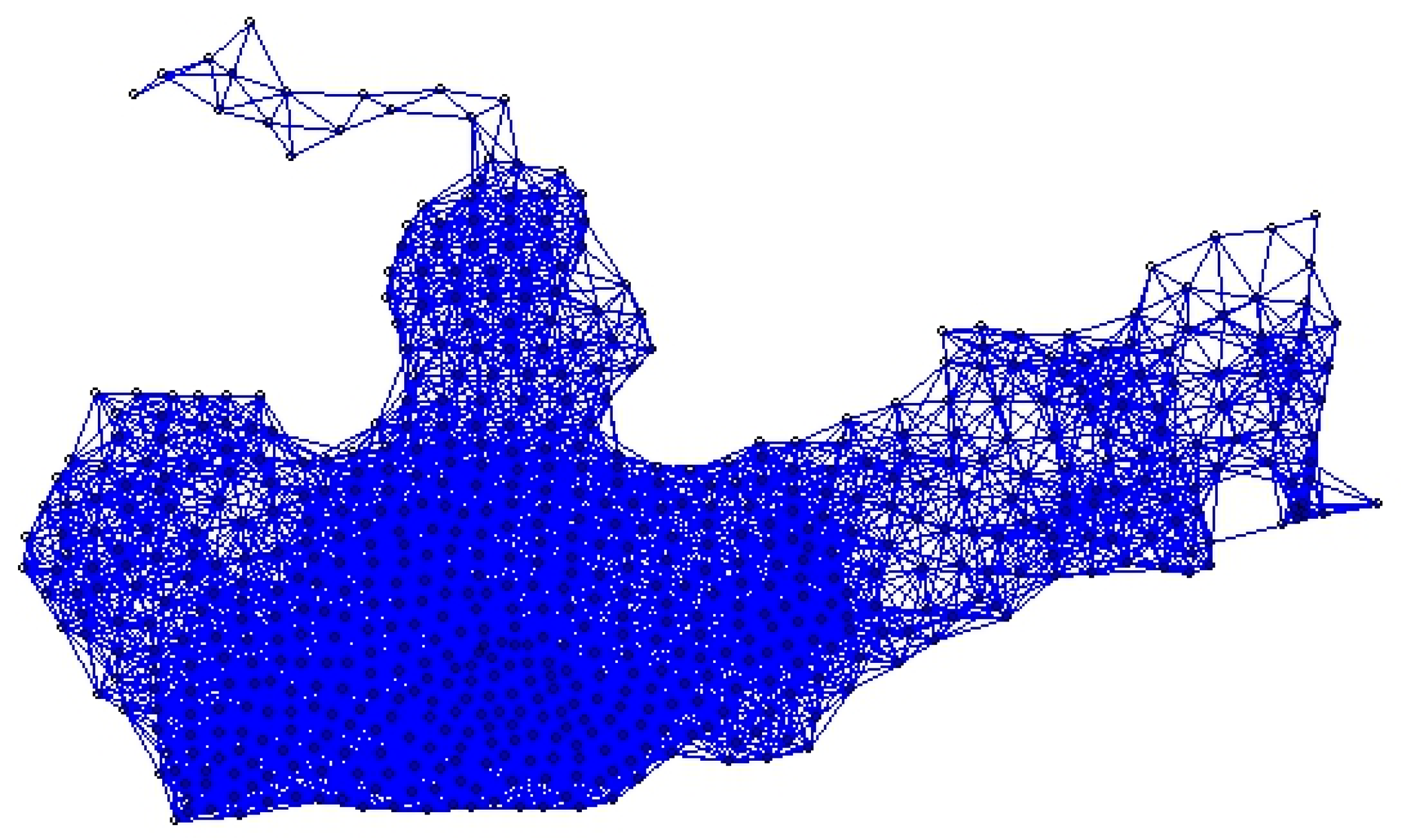
Figure 6.
Connectivity graph of the rustbelt states.

Table 1.
Dependent and independent variables.
| Variable | Meaning |
|---|---|
| Y | Republican’s share of the vote in the U.S. presidential election (https://github.com/tonmcg/US_County_Level_Election_Results_08-20/blob/f9b5f335ad1c66a7eba681539db49eec0c22787b/2020_US_County_Level_Presidential_Results.csv (accessed on 30 April 2021)). |
| ALWAYS | the share of respondents who thought they often wore face masks (https://github.com/nytimes/covid-19-data (accessed on 30 April 2021)). |
| Housi_Unit | The number of housing units |
| Education | The number of residents who are high school graduates or above |
| Urate | Unemployment rate |
| income | Household income |
| deaths | COVID-19 Death Tolls |
| cases | COVID-19 cases |
Table 2.
Descriptive statistics of dependent and independent variables.
| Variable | N | Mean | St. Dev | Min. | Max. |
|---|---|---|---|---|---|
| Y | 669 | 0.662 | 0.127 | 0.120 | 0.900 |
| ALWAYS | 669 | 0.536 | 0.139 | 0.190 | 0.880 |
| Housi_Unit | 669 | 52,630.64 | 135,268.2 | 1107 | 2,204,019 |
| Education | 669 | 34,032.23 | 84,810.53 | 616 | 1,314,995 |
| Urate | 669 | 4.591 | 1.273 | 2.400 | 13.00 |
| income | 669 | 52,867.07 | 12,235.31 | 26,278 | 115,301 |
| deaths | 669 | 71.175 | 306.17 | 0 | 5517 |
| cases | 669 | 2487 | 9336.54 | 0 | 198,184 |
Table 3.
AIC values of Spatial Regression Models. (COVID-19 cases as the independent variable).
| Spatial Regression Models | AIC |
|---|---|
| GNS Model | 1186.7 |
| SAC | 1237.6 |
| Spatial Durbin Model | 1185.7 |
| Spatial Durbin Error Model | 1187.9 |
| Spatial lag model | 1247.8 |
| Spatial error model | 1235.6 |
Table 4.
Estimates of Spatial Durbin Model. (COVID-19 cases as the independent variable).
| Variable | Estimate | Std. Error | p-Value |
|---|---|---|---|
| (Intercept) | 0.0009 | 0.021 | 0.964 |
| Housi_Unit | −1.000 | 0.115 | <0.0001 *** |
| Education | 0.393 | 0.109 | 0.0003 *** |
| Urate | 0.067 | 0.036 | 0.069 |
| Income | 0.007 | 0.038 | 0.847 |
| cases | 0.290 | 0.051 | <0.0001 *** |
| ALWAYS | −0.347 | 0.043 | <0.0001 *** |
| lag.Housi_Unit | 0.306 | 0.174 | 0.079 |
| lag.Education | −0.067 | 0.151 | 0.659 |
| lag.Urate | −0.093 | 0.044 | 0.033 * |
| lag.Income | −0.302 | 0.048 | <0.001 *** |
| lag.cases | −0.034 | 0.062 | 0.579 |
| lag.ALWAYS | 0.105 | 0.049 | 0.032 * |
Significant codes: 0.001 ***; 0.05 *.
Table 5.
AIC values of Spatial Regression Models. (COVID-19 deaths as the independent variable).
| Spatial Regression Models | AIC |
|---|---|
| GNS Model | 1189.6 |
| SAC | 1237.2 |
| Spatial Durbin Model | 1189 |
| Spatial Durbin Error Model | 1189.1 |
| Spatial lag model | 1243.1 |
| Spatial error model | 1235.6 |
Table 6.
Estimates of Spatial Durbin Model (COVID-19 deaths as the independent variable).
| Variable | Estimate | Std. Error | p-Value |
|---|---|---|---|
| (Intercept) | 0.0009 | 0.021 | 0.965 |
| Housi_Unit | −0.891 | 0.110 | <0.0001 *** |
| Education | 0.333 | 0.109 | 0.002 |
| Urate | 0.061 | 0.037 | 0.100 |
| Income | 0.009 | 0.038 | 0.807 |
| deaths | 0.253 | 0.045 | <0.0001 *** |
| ALWAYS | −0.342 | 0.043 | <0.0001 *** |
| lag.Housi_Unit | 0.318 | 0.168 | 0.058 |
| lag.Education | −0.110 | 0.148 | 0.458 |
| lag.Urate | −0.089 | 0.044 | 0.043 * |
| lag.Income | −0.294 | 0.048 | <0.001 *** |
| lag.deaths | −0.038 | 0.054 | 0.479 |
| lag.ALWAYS | 0.090 | 0.049 | 0.068 |
Significant codes: 0.001 ***; 0.05 *.
Table 7.
Direct and indirect effects from Spatial Durbin Model (in Z values, COVID-19 cases as the independent variable).
Table 7.
Direct and indirect effects from Spatial Durbin Model (in Z values, COVID-19 cases as the independent variable).
| Variable | Direct | Indirect | Total |
|---|---|---|---|
| Housi_Unit | −7.776 *** | −0.190 | −3.170 ** |
| Education | 3.275 *** | 0.427 | 1.668 |
| Urate | 1.663 | −1.894 | −0.746 |
| Income | −0.972 | −6.712 *** | −6.577 *** |
| cases | 5.791 *** | 1.148 | 4.424 *** |
| ALWAYS | −8.462 *** | −0.342 | −8.510 *** |
Significant codes (p-value): 0.001 ***; 0.01 **
Table 8.
Direct and indirect effects from Spatial Durbin Model (in Z values, COVID-19 deaths as the independent variable).
Table 8.
Direct and indirect effects from Spatial Durbin Model (in Z values, COVID-19 deaths as the independent variable).
| Variable | Direct | Indirect | Total |
|---|---|---|---|
| Housi_Unit | −7.237 *** | 0.081 | −2.723 ** |
| Education | 2.727 ** | 0.033 | 1.169 |
| Urate | 1.509 | −1.855 | −0.791 |
| Income | −0.858 | −6.739 *** | −6.478 *** |
| deaths | 5.608 *** | 0.956 | 4.176 *** |
| ALWAYS | −8.401 *** | −0.667 | −8.803 *** |
Significant codes (p-value): 0.001 ***; 0.01 **.
Disclaimer/Publisher’s Note: The statements, opinions and data contained in all publications are solely those of the individual author(s) and contributor(s) and not of MDPI and/or the editor(s). MDPI and/or the editor(s) disclaim responsibility for any injury to people or property resulting from any ideas, methods, instructions or products referred to in the content. |
© 2023 by the author. Licensee MDPI, Basel, Switzerland. This article is an open access article distributed under the terms and conditions of the Creative Commons Attribution (CC BY) license (https://creativecommons.org/licenses/by/4.0/).
Share and Cite
MDPI and ACS Style
Wu, S. The Spatial Data Analysis of Determinants of U.S. Presidential Voting Results in the Rustbelt States during the COVID-19 Pandemic. ISPRS Int. J. Geo-Inf. 2023, 12, 212. https://doi.org/10.3390/ijgi12060212
AMA Style
Wu S. The Spatial Data Analysis of Determinants of U.S. Presidential Voting Results in the Rustbelt States during the COVID-19 Pandemic. ISPRS International Journal of Geo-Information. 2023; 12(6):212. https://doi.org/10.3390/ijgi12060212
Chicago/Turabian StyleWu, Shianghau. 2023. "The Spatial Data Analysis of Determinants of U.S. Presidential Voting Results in the Rustbelt States during the COVID-19 Pandemic" ISPRS International Journal of Geo-Information 12, no. 6: 212. https://doi.org/10.3390/ijgi12060212
Note that from the first issue of 2016, this journal uses article numbers instead of page numbers. See further details here.