Volatility Spillover Effects in the Moroccan Interbank Sector before and during the COVID-19 Crisis

Abstract

The objective of this paper is to analyze the volatility spillover effects in the Moroccan interbank sector before and during the COVID-19 pandemic crisis using the DY model. Specifically, this study assesses the impact of the recent COVID-19 outbreak on the transmission of volatility among Moroccan banks listed in the Moroccan stock market. The data sample frequency is daily and extends from 1 January 2012 to 31 December 2021, excluding holidays. The empirical results indicate that the volatility spillover index increased during the pandemic crisis. We also found varying degrees of interdependence and spillover effects between the six publicly traded Moroccan banks and the Moroccan banking sector stock index before and during the COVID-19 pandemic crisis.

1. Introduction

A successive particular events, namely the COVID-19 health crisis and the Russian military offensive in Ukraine, have threatened the financial economic stability of countries such as Morocco by plunging expectations for economic recovery into a spiral of uncertainty.

The COVID-19 pandemic started as a health emergency and quickly turned into a global social and economic disaster. The impact of the pandemic seems to vary by sector, with a very different impact in the banking sector. However, the prolonged freezes, loan deferrals, and uncertain political outlook have increased the systemic vulnerability of the banking sector. According to the experts, “vulnerabilities in credit markets, emerging markets, and banks could even trigger a new financial crisis”.

The Moroccan government carried out a number of steps, the most important of which was putting in place containment at the beginning of 2020, in order to learn from what other countries had done to fight this virus.

This decision reduced the number of contaminations throughout the containment, but it had unmistakable consequences for the country’s economic and financial performance.

The period we have chosen in our study is characterized by high volatility due to the evolution of the pandemic crisis COVID-19 and the measures taken by the health authorities, which will allow us to analyze the impact of the epidemic crisis on the banking sector.

The partial halt of economic activity in the world through the containment decisions to counteract the pandemic COVID-19 has impacted all sectors of activity.

Researchers at the international level in all fields, especially in the economy, are now rushing to assess the effects of COVID-19 on the real economy and draw conclusions in order to seek optimal solutions.

The idea here is to use the approaches developed by Diebold and Yilmaz (2012, 2014) to analyze the impact of the evolution of the epidemic on the transmission of volatility between the financial institutions composing the Moroccan interbank system. Specifically, we will determine the extent to which the volatility of a bank’s return is influenced by foreign shocks from other banks and the banking sector index, respectively, by assuming that there are three sources of shocks: internal, external from another financial institution, and external from the market.

These approaches allowed us to identify the systemic and financial contagion risk of publicly traded Moroccan banks through volatility spillover effects, and we determined how banks communicate contagion risk during the COVID-19 pandemic. The health crisis has contributed to the increase in systemic risk vulnerabilities of the financial system’s interconnected financial institutions.

This research was motivated by this problem and allowed us to rank individual Moroccan banks in terms of their systemic importance based on the magnitude of their contribution to volatility spillover effects before and during the crisis. We also calculated the total spillover index before and during the crisis.

Using daily data over the period from 1 January 2012 to 31 December 2021, we show herein how the events related to the epidemic health crisis affected the systemic risk in the Moroccan banking system.

2. Literature Review

In recent decades, especially after the 2008 global financial crisis, the term “financial contagion” was been the basis for several research studies on the transmission of financial crises. King and Wadhwani (1990) were the first researchers to address contagions by examining the effects of the 1987 stock market crash. Other subsequent studies have developed the modeling of a financial contagion.

The concept of a financial contagion has been studied using correlation (Baig and Goldfajn 1999; Calvo and Reinhart 1996; Adam et al. 1996; Edwards and Susmel 2001).

Forbes and Rigobon (2001) argue that “standard tests” for contagion produce insignificant results due to heteroscedasticity, endogeneity, or omitted variable problems. They argue that studies that address these problems find interdependence, but not contagion.

The spillover index, proposed by Diebold and Yilmaz (2009), measures the interdependence of returns and volatilities using the p-order VAR model with N variables and an H-period forecast. This index aggregates the contribution of each variable to the variance of the forecast error of the other variables over multiple returns. Yilmaz (2010) examined The Spillover of Volatility on East Asian Stock Markets and showed the existence of spillover dynamics in the behavior of the East Asian return and volatility spillover indices over time, and showed that the return spillover index reveals increased integration among East Asian stock markets while the volatility spillover index experiences significant spikes during crises.

Diebold and Yilmaz (2012) used the generalized vector autoregression VAR that produces VAR ordering invariant estimates to compute volatility spillovers to characterize daily volatility spillovers in U.S. equity, bond, foreign exchange, and commodity markets from January 1999 to September 2009. They showed large swings in market volatility and that volatility spillovers to other markets also increased during the global financial crisis that began in 2007, after being quite limited before the crisis.

Diebold and Yilmaz (2014) used vector autoregression (VAR) analyses to figure out how U.S. financial institutions affect each other.

To construct a volatility connectivity index, Demirer et al. (2018) applied the methodology of Diebold and Yilmaz (2014) to the daily stock prices of the 40 largest U.S. financial institutions to construct a volatility index. Then, they figured out how sensitive each U.S. nonfinancial firm’s performance at the time was to this index.

To study the impact of the COVID-19 pandemic crisis on financial market interdependence, Shahzad et al. (2021) analyzed the connectivity among 95 U.S. firms between 2018 and 2020, and detected a spike in the level of risk contagion during the COVID-19 pandemic.

Mahdi Moradi et al. (2021) investigated the effects of macroeconomic variables on the risk of stock price decline under the conditions of economic uncertainty in the Iranian market. Their study examines the significant relationship between some firm characteristics and stock price decline. The research model was estimated using a fixed effect model, and the DUVOL (down-to-up volatility) measure is defined as a proxy for the risk of stock price fall. Their results show that there is a positive association between inflation and unemployment rates and the risk of stock price crashes, while GDP and exchange rates are negatively correlated with the risk of crashes.

Sadowski et al. (2021) investigated global mobility during the lockdowns of the COVID-19 pandemic. Their study highlights a time lag between the two applied databases, Google Mobility and John Hopkins University, influencing correlations between mobility and pandemic development. Their studies show that the number of new COVID-19 cases increased since containment was put in place.

3. Data and Methodology

3.1. Data

In this paper, we apply the spillover index on a daily series of log-returns of the Moroccan banking sector index and the stocks of the six listed Moroccan banks: Attijari-Wafa-Bank (ATW), Popular Bank (BCP), Moroccan Bank for International Trade (BMCI), Bank of Africa (BMCE), Loan Estate and Hotel Bank (CIH), and Moroccan mortgage loan (CDM), see Supplementary Material Table S1.

The period we have chosen in our document is from 1 January 2012 to 31 December 2021. Since the stock markets are closed on weekends and holidays, non-business days are not taken into account.

Our database is subdivided into two sub-periods:

–

The period before the COVID-19 crisis: From 1 January 2012 to 31 December 2019;

–

The period during the COVID-19 crisis: From 1 January 2020 to 31 December 2021.

3.2. Methodology

Our study consists of the evaluation and analysis of the transmission of volatility spillovers between the six listed Moroccan banks and the Moroccan banking sector index. To do this, we addressed the main approaches of Diebold and Yilmaz (2012, 2014).

The evolution over time of the return and volatility of an asset is due either to internal shocks (its own shocks) or to external shocks from other assets. Thus, the goal is to figure out, for each asset, how much of the total expected variance comes from the two types of shocks.

In our paper, we apply a method developed by Diebold and Yilmaz (2012, 2014). This method is based on p-order VAR (generalized vector autoregression) models.

The advantage of this approach is that this vector produces generalized, order-invariant variance decompositions, which allows for correlated shocks but accounts for correlation appropriately instead of orthogonalizing shocks.

3.2.1. $VAR\left(p\right)$ Model

A multivariate vector autoregressive stochastic process of order p, denoted$VAR\left(p\right)$, is a generalization of the univariate autoregressive stochastic process $AR\left(p\right)$. The dimension of the $VAR\left(p\right)$ process is (N × 1), where N is the number of variables studied.

The time course for each variable is modeled by an equation as a function of the time-lagged values of that variable, the lagged values of the other variables in the model, and an error term.

For a $VAR\left(p\right)$ model, each financial variable is modeled as a linear combination of its past values and the past values of the other financial variables in the system. Since we have a database of several time series that impact each other, they were modeled as a system of linear equations where the number of equations corresponds to the number of financial variables.

If not, we will have a system of N linear equations for N time series that affect each other.

A model $VAR\left(p\right)$ for N processes $\left({(X_{1,t})}_{tϵ\mathbb{Z}},{(X_{2,t})}_{tϵ\mathbb{Z}}\dots \dots \dots \dots {(X_{N,t})}_{tϵ\mathbb{Z}}\right)$ is presented as a system of N linear equations as follows:

$$\{\begin{array}{c}{X}_{1,t}=c_1+\left[{\mathsf{\Phi }}_{11,1}{X}_{1,t-1}+{\mathsf{\Phi }}_{12,1}{X}_{2,t-1}+\dots +{\mathsf{\Phi }}_{1N,1}{X}_{N,t-1}\right]+\dots +\left[{\mathsf{\Phi }}_{11,p}{X}_{1,t-p}+{\mathsf{\Phi }}_{12,p}{X}_{2,t-p}+\dots +{\mathsf{\Phi }}_{1N,p}{X}_{N,t-p}\right]+{\epsilon }_{1,t}\\ X_{2,t}=c_2+\left[{\mathsf{\Phi }}_{21,1}{X}_{1,t-1}+{\mathsf{\Phi }}_{22,1}{X}_{2,t-1}+\dots +{\mathsf{\Phi }}_{2N,1}{X}_{N,t-1}\right]+\dots +\left[{\mathsf{\Phi }}_{21,p}{X}_{1,t-p}+{\mathsf{\Phi }}_{22,p}{X}_{2,t-p}+\dots +{\mathsf{\Phi }}_{2N,p}{X}_{N,t-p}\right]+{\epsilon }_{2,t}\\ .\\ .\\ .\\ X_{N,t}=c_N+\left[{\mathsf{\Phi }}_{N1,1}{X}_{1,t-1}+{\mathsf{\Phi }}_{N2,1}{X}_{2,t-1}+\dots +{\mathsf{\Phi }}_{NN,1}{X}_{N,t-1}\right]+\dots +\left[{\mathsf{\Phi }}_{N1,p}{X}_{1,t-p}+{\mathsf{\Phi }}_{N2,p}{X}_{2,t-p}+\dots +{\mathsf{\Phi }}_{NN,p}{X}_{N,t-p}\right]+{\epsilon }_{N,t}\end{array}$$

A generalized $VAR\left(p\right)$ model can be presented in matrix form as follows:

$$\begin{gathered} X_t=C+{\displaystyle \sum }_{k=1}^p{A}_k{X}_{t-k}+{\epsilon }_t=C+A_1{X}_{t-1}+A_2{X}_{t-2}+\dots +A_p{X}_{t-p}+{\epsilon }_t \\ \left(\begin{array}{c}{X}_{1,t}\\ X_{2,t}\\ ⋮\\ X_{N,t}\end{array}\right)=\left(\begin{array}{c}{c}_1\\ c_2\\ ⋮\\ c_N\end{array}\right)+[\left(\begin{array}{cccc}{\mathsf{\Phi }}_{11,1}& {\mathsf{\Phi }}_{12,1}& \cdots & {\mathsf{\Phi }}_{1N,1}\\ {\mathsf{\Phi }}_{21,1}& {\mathsf{\Phi }}_{22,1}& \cdots & {\mathsf{\Phi }}_{2N,1}\\ ⋮& ⋮& \ddots & ⋮\\ {\mathsf{\Phi }}_{N1,1}& {\mathsf{\Phi }}_{N2,1}& \cdots & {\mathsf{\Phi }}_{NN,1}\end{array}\right)\left(\begin{array}{c}\begin{array}{c}{X}_{1,t-1}\\ X_{2,t-1}\\ ⋮\end{array}\\ X_{N,t-1}\end{array}\right)+\cdots +\left(\begin{array}{cccc}{\mathsf{\Phi }}_{11,p}& {\mathsf{\Phi }}_{12,p}& \cdots & {\mathsf{\Phi }}_{1N,p}\\ {\mathsf{\Phi }}_{21,p}& {\mathsf{\Phi }}_{22,p}& \cdots & {\mathsf{\Phi }}_{2N,p}\\ ⋮& ⋮& \ddots & ⋮\\ {\mathsf{\Phi }}_{N1,p}& {\mathsf{\Phi }}_{N2,p}& \cdots & {\mathsf{\Phi }}_{NN,p}\end{array}\right)\left(\begin{array}{c}\begin{array}{c}{X}_{1,t-p}\\ X_{2,t-p}\\ ⋮\end{array}\\ X_{N,t-p}\end{array}\right)]+\left(\begin{array}{c}{\epsilon }_{1,t}\\ {\epsilon }_{2,t}\\ ⋮\\ {\epsilon }_{N,t}\end{array}\right) \end{gathered}$$

where

• $C—\mathrm{vector}\left(N\times 1\right)\mathrm{of}\mathrm{the}N \mathrm{constants}{c}_i\mathrm{of}\mathrm{the}\mathrm{equasionts}\mathrm{of}\mathrm{the}VAR\left(p\right)\mathrm{model}$;
• $X_t—\mathrm{vector}\left(N\times 1\right)\mathrm{of}\mathrm{the}N\mathrm{variables}{X}_{i,t}\mathrm{of}\mathrm{the}VAR\left(p\right)\mathrm{model}$;
• ${\epsilon }_t—\mathrm{vector}\left(N\times 1\right)\mathrm{of}\mathrm{the}N\mathrm{innovations}\mathrm{of}\mathrm{the}VAR\left(p\right) \mathrm{model}$;
• $A_k—\mathrm{matrix}\left(N\times N\right)\mathrm{of}\mathrm{the}\mathrm{coefficients}\mathrm{of}\mathrm{the}VAR\left(p\right)\mathrm{model}$;
• $X_{t-k}—\mathrm{vector}\left(N\times 1\right)\mathrm{of}\mathrm{the}N\mathrm{variables}{X}_{i,t}\mathrm{lagged}\mathrm{at}\mathrm{order}k.$

3.2.2. Volatility of Returns

There are many measures of return of a stock index; a frequently used one is the geometric return or the log-return, which involves calculating the logarithm of the differential of the values in t and (t − 1).

The return of this stock at time t is defined as follows:

$$R_t=\log \left(\frac{P_t}{P_{t-1}}\right)=\log \left(P_t\right)-\log \left(P_{t-1}\right)=\log \left(r_t+1\right)\mathrm{where}t=1,2,\dots ,n$$

and

$$r_t=\frac{P_t-P_{t-1}}{P_{t-1}}$$

where

• $R_t—$the log-return of a stock at time t;
• $r_t—$the algebraic return of a stock at time t;
• $P_t—$the stock price at time t.

We often consider daily log returns when analyzing our financial series. To estimate the volatility of assets, there are several methods in the financial literature. Garman and Klass (1980) used the information of the day based on historical daily prices (opening, closing, high and low prices) to estimate the volatility of financial series. For the famous GARCH family (Engle and Kroner 1995; Engle and Sheppard 2001; Engle 2002; Francq and Zakoian 2010), these models use the prior information of stock prices. The approach proposed in this paper is Parkinson (1980), which gives an estimate of the variance of returns based on the highest prices $(H_i)$ and the lowest prices $(L_i)$.

The Parkinson’s volatility is then obtained by the following formula:

$${\tilde{\sigma }}_{it}^2=0.361\times {(\ln \left(H_{it}\right)-\ln \left(L_{it}\right))}^2$$

3.2.3. Decomposition of the Variance of the Forecast Error (FEVD)

Given a $VAR\left(p\right)$ model with N variables, the decomposition of the variance of the forecast error of the variable $X_{i,t}$ determines the percentage of the variance of this error that is explained by a shock to another variable $X_{j,t}$. The variance of the forecast error of i represents 100%, and each variable j of the system of its $VAR\left(p\right)$ model will make a contribution to explain this variance.

The forecast error variance decomposition (FEVD) is used to indicate how much information each variable contributes to the other variables in the $VAR\left(p\right)$ model. It finds out how much the forecast error variance of each variable can be explained by shocks to the other variables that come from the outside.

Diebold and Yilmaz (2012) calculate the forecast error variance decompositions as follows:

$$d_{ij}^H=\frac{{\mathsf{\sigma }}_{jj}^{-1}{\mathsf{\Sigma }}_{h=0}^{H-1}{\left(e_i^{\prime }{A}_h{\mathsf{\Sigma }e}_j\right)}^2}{{\mathsf{\Sigma }}_{h=0}^{H-1}(e_i^{\prime }{A}_h{\mathsf{\Sigma }A}_h^{\prime }{e}_i)}$$

where

• $d_{ij}^H$ explains the shocks contributed by the financial variable $X_j$ to the variance of the forecast error of another variable$X_i$;
• ${\sigma }_{jj}$—standard deviation of the residual for the $j^{\mathrm{th}}$ equation in the model;
• $e_i$—selection vector, with one for the $i^{\mathrm{th}}$ element and zeros otherwise;
• $\mathsf{\Sigma }$—vector of variances of the $\epsilon$ disturbances.

The individual row sum of $d_{ij}\left(H\right)$ is not equal to unity $\left({\mathsf{\Sigma }}_{j=1}^N{d}_{ij}^g\ne 1\right)$. Therefore, the row sum result is used to divide the individual component of the decomposition matrix to normalize it. This is expressed by the following calculation:

$${\widetilde{ d}}_{ij}^H=\frac{d_{ij}^H}{{\mathsf{\Sigma }}_{j=1}^N{d}_{ij}^H}$$

where

• $d_{ij}^H$—the proportion of shocks contributed by the financial variable $X_j$ to the variance of the forecast error of another variable$X_i$;
• ${\mathsf{\Sigma }}_{j=1}^N{\widetilde{d }}_{ij}^H=1$.

3.2.4. Spillover Index

The total spillover index determines the contribution of volatility shocks of all variables to the total variance of forecast errors:

$$S^H=\frac{{\mathsf{\Sigma }}_{i,j=1,i\ne j}^N{\tilde{d}}_{ij}^H}{{\mathsf{\Sigma }}_{i,j=1}^N{\tilde{d}}_{ij}^H}\times 100=\frac{{\mathsf{\Sigma }}_{i,j=1,i\ne j}^N{\tilde{d}}_{ij}^H}{N}\times 100\mathrm{with}i\ne j$$

The directional spillovers received by institution i from all other institutions j (from others) are $S_{i \overleftarrow{from} j}^H=\frac{{\mathsf{\Sigma }}_{i,j=1,i\ne j}^N{\tilde{d}}_{ij}^H}{{\mathsf{\Sigma }}_{j=1}^N{\tilde{d}}_{ij}^H}\times 100$.

The directional spillovers transmitted by institution i to all other institutions j (to others) are $S_{i \overrightarrow{to} j}^H=\frac{{\mathsf{\Sigma }}_{j=1,i\ne j}^N{\tilde{d}}_{ij}^H}{{\mathsf{\Sigma }}_{j=1}^N{\tilde{d}}_{ij}^H}\times 100$.

The difference between the gross shocks sent from asset i and the gross shocks received from all other assets can be used to figure out the net spillovers from asset i to all other assets:

$$NS=S_{i \overrightarrow{to} j}^H-S_{i \overleftarrow{from} j}^H$$

The Diebold–Yilmaz variance decomposition table is shown below (

Table 1. Variance decomposition of Diebold and Yilmaz.

	${\mathit{X}}_1$	${\mathit{X}}_2$	$\dots$	${\mathit{X}}_{\mathit{N}}$	Contribution from Others
$X_1$	$d_{11}\left(H\right)$	$d_{12}\left(H\right)$	$\dots$	$d_{1N}\left(H\right)$	${\mathsf{\Sigma }}_{j=1}^N{d}_{1j}\left(H\right)j\ne 1$
$X_2$	$d_{21}\left(H\right)$	$d_{22}\left(H\right)$	$\dots$	$d_{2N}\left(H\right)$	${\mathsf{\Sigma }}_{j=1}^N{d}_{1j}\left(H\right)j\ne 2$
$⋮$	$⋮$	$⋮$	$\ddots$	$⋮$	$⋮$
$X_N$	$d_{N1}\left(H\right)$	$d_{N2}\left(H\right)$	$\dots$	$d_{NN}\left(H\right)$	${\mathsf{\Sigma }}_{j=1}^N{d}_{Nj}\left(H\right)j\ne N$
Contribution to others	${\mathsf{\Sigma }}_{i=1}^N{d}_{i1}\left(H\right)$ $i\ne 1$	${\mathsf{\Sigma }}_{i=1}^N{d}_{i2}\left(H\right)$ $i\ne 2$	$\dots$	${\mathsf{\Sigma }}_{i=1}^N{d}_{i3}\left(H\right)$ $i\ne 3$	$\frac{1}{N}{\mathsf{\Sigma }}_{i,j=1}^N{d}_{ij}\left(H\right)i\ne j$

), wherein we present the underlying variance decomposition based on a daily VAR, identified using the generalized variance decomposition of KPPS. In addition, the $i{j}^{\mathrm{th}}$ entry is the estimated contribution to the variance of the H-day forecast error of bank i due to shocks from bank j. The first row shows assets from which the spillovers emanate. The first column refers to the assets that receive the spillovers. The column “From Others” shows the sum of the spillovers received by the asset listed in the first column. The row “Contribution to Others” is the sum of the spillovers from the asset listed in the first row.

The “Net Volatility Spillover” row gives the difference in total directional spillovers (“Contribution to others” minus “From others”). The total spillover index is the sum of all the columns and rows that are not on the diagonal compared to the sum of all the columns and rows that are on the diagonal, expressed as a percentage.

The advantage of using this method lies in the dynamic modeling of the overflow, taking into account the temporal variations.

4. Preliminary Analysis

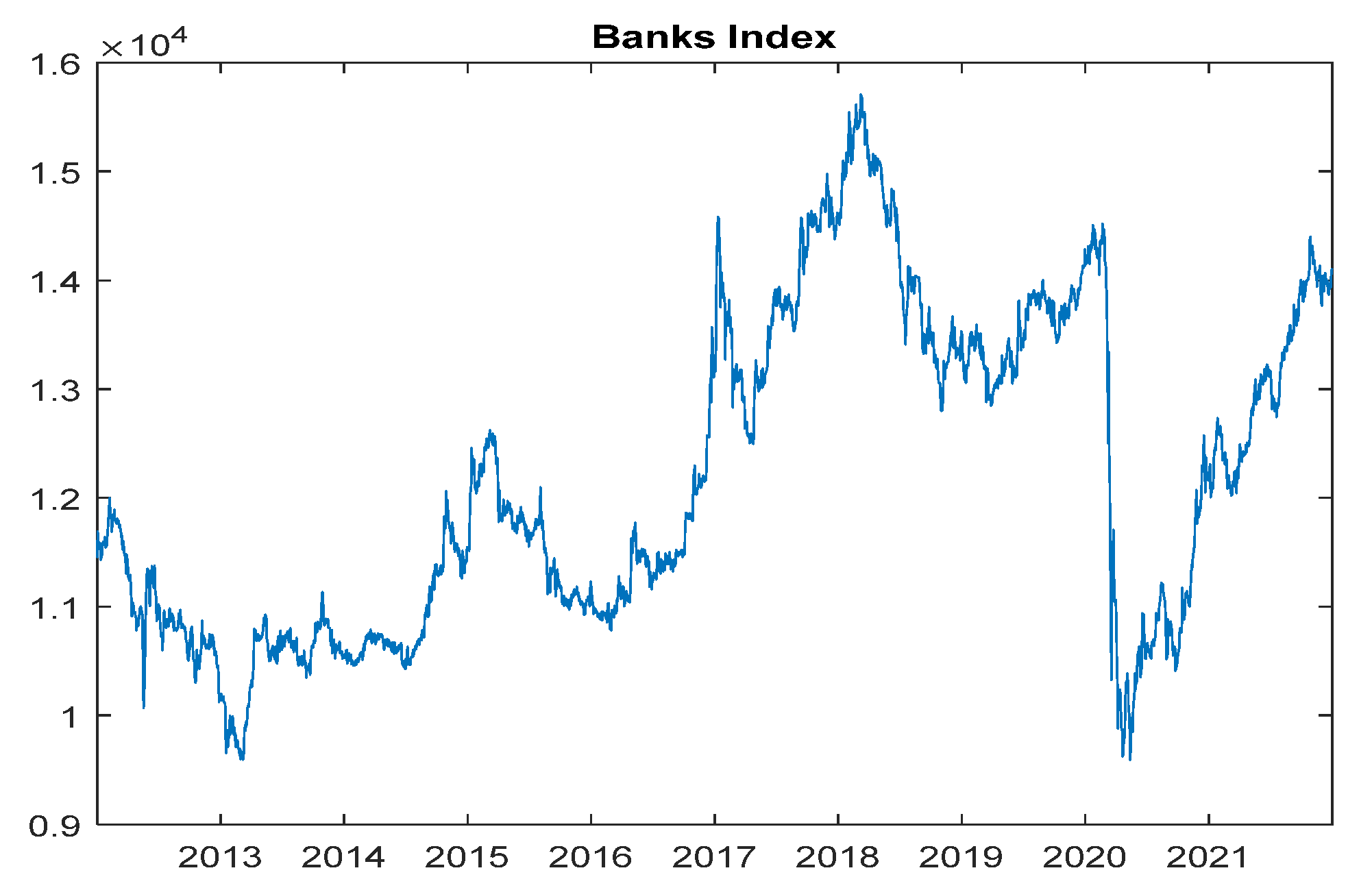
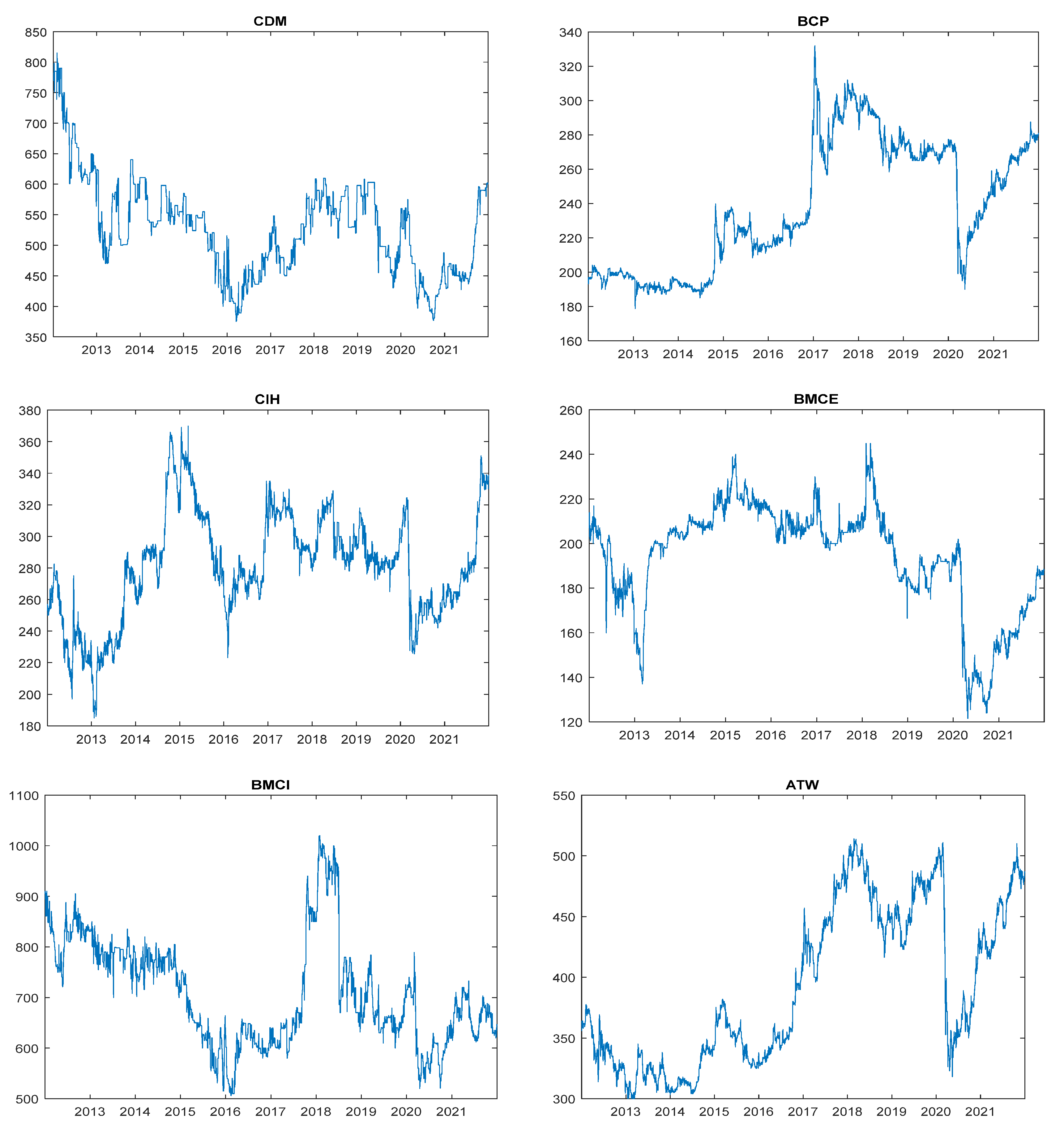
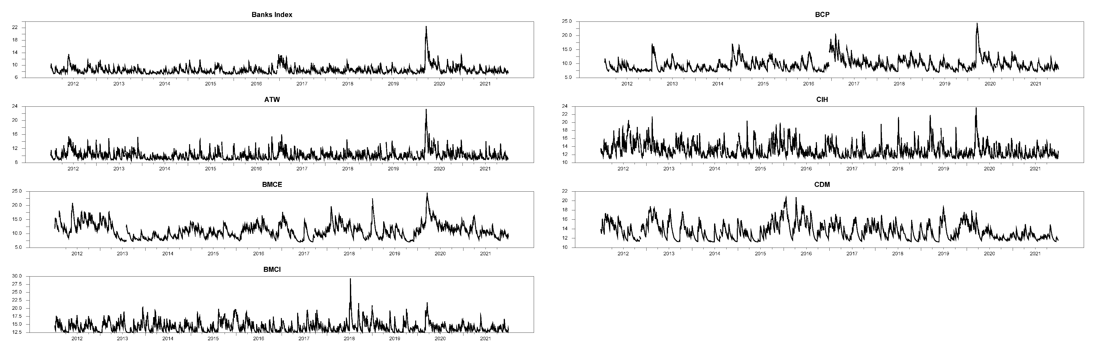
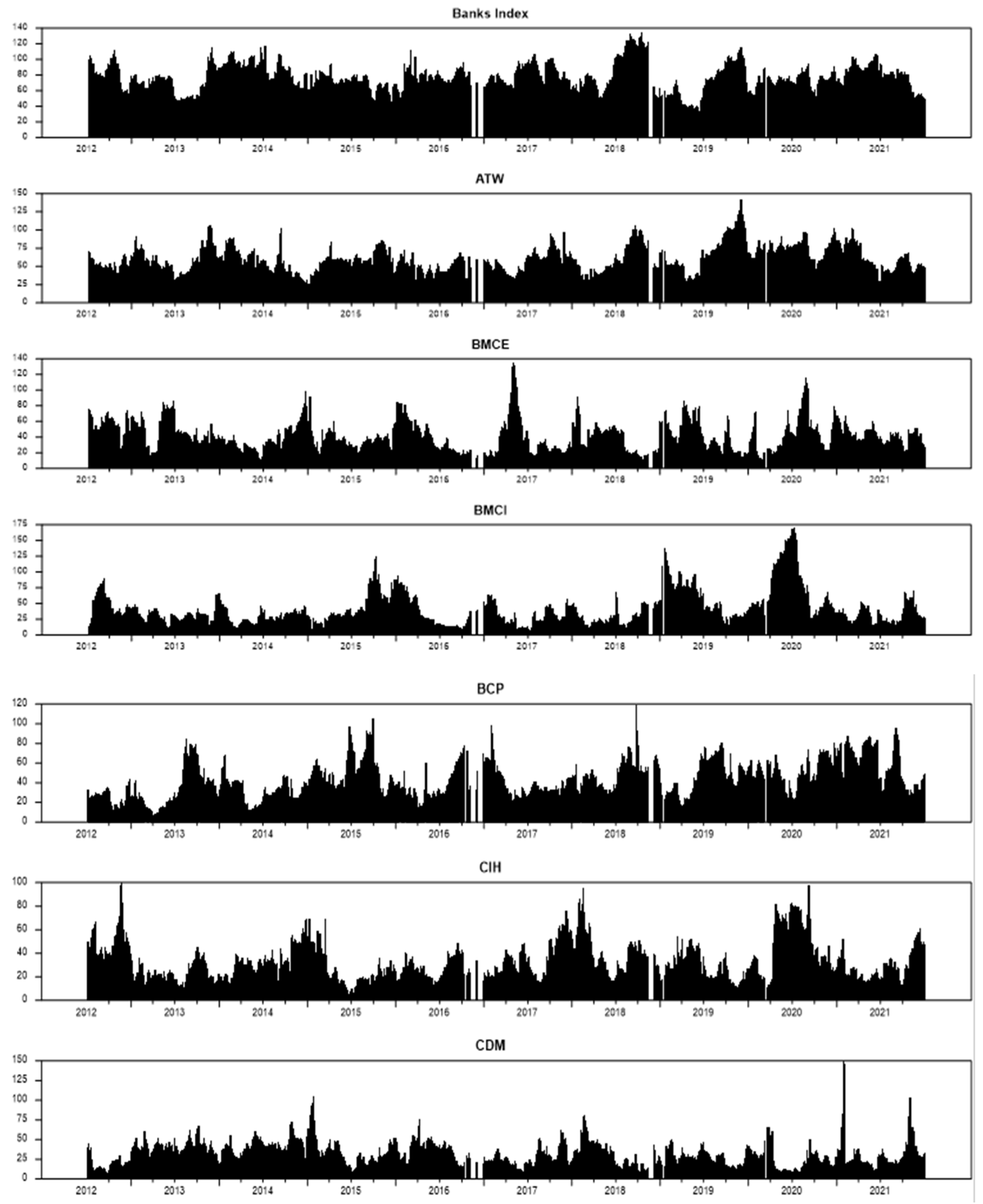
By analyzing the evolution of the value of the banking sector index and the values of the six banks constituting our sample during the period of the pandemic crisis presented in Figure 1 and Figure 2, we noticed that these stock prices were affected by the effects of the health crisis at the beginning of the year 2020. We noted that these graphs are characterized by a downward trend during the first months of 2020 (period of the appearance of the first cases of COVID-19 in Morocco), followed by a partial recovery at the end of 2020 and during the year 2021.

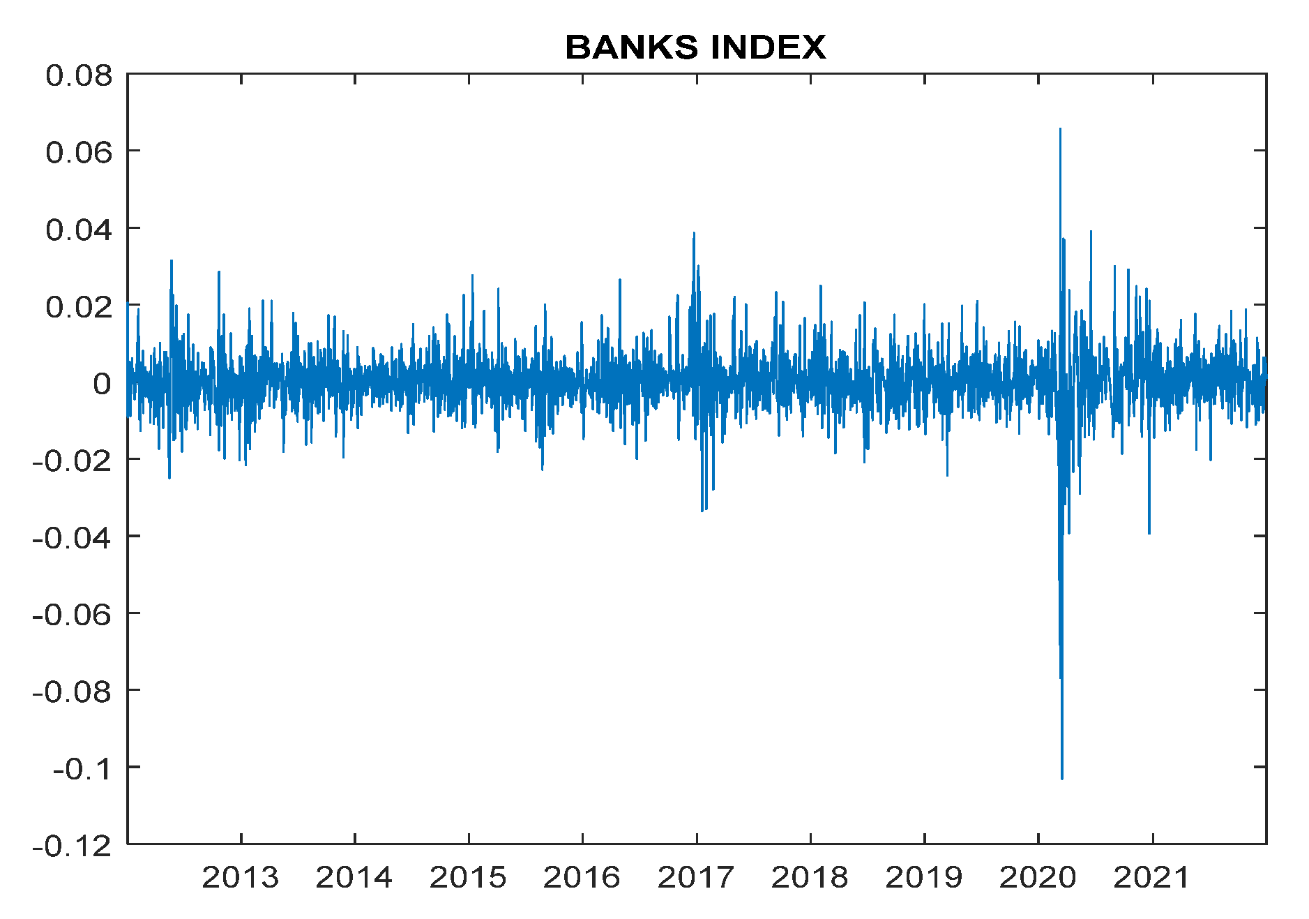
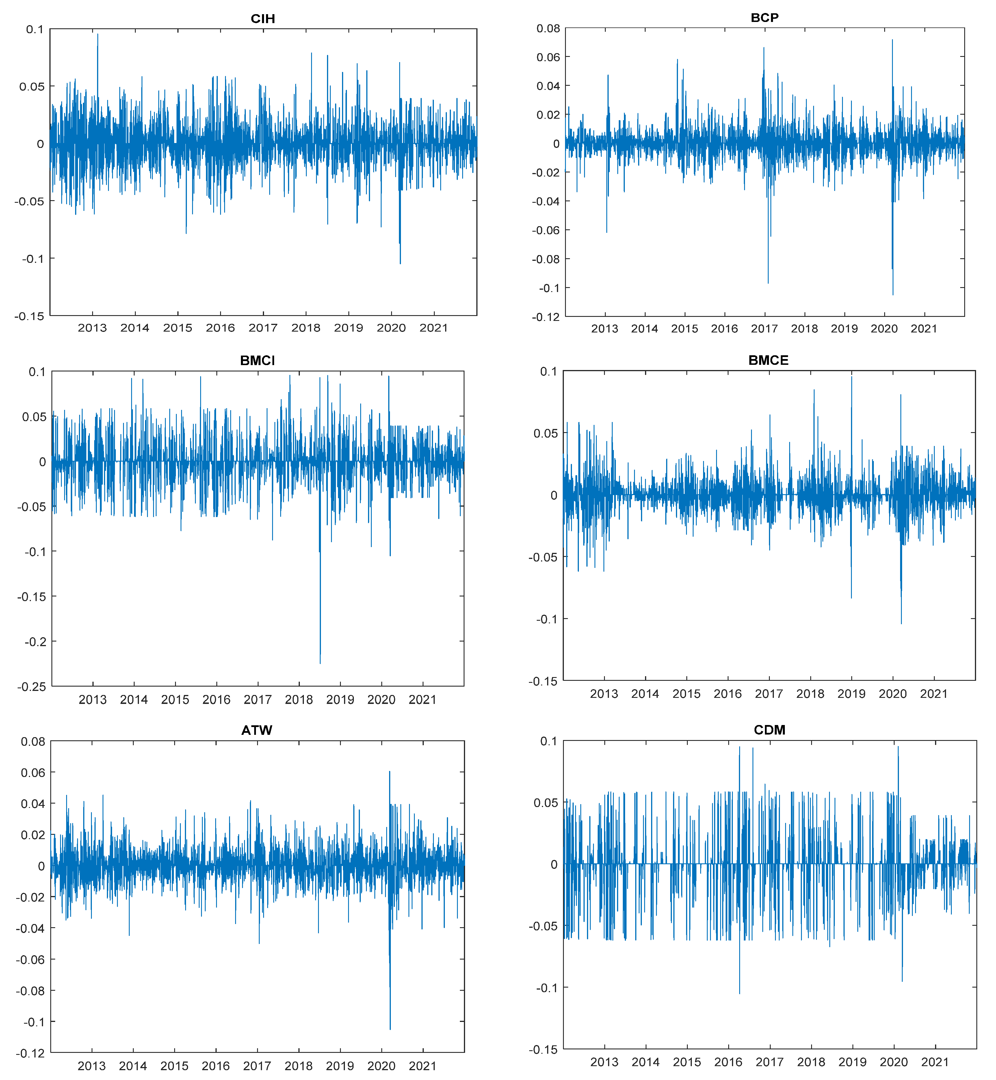
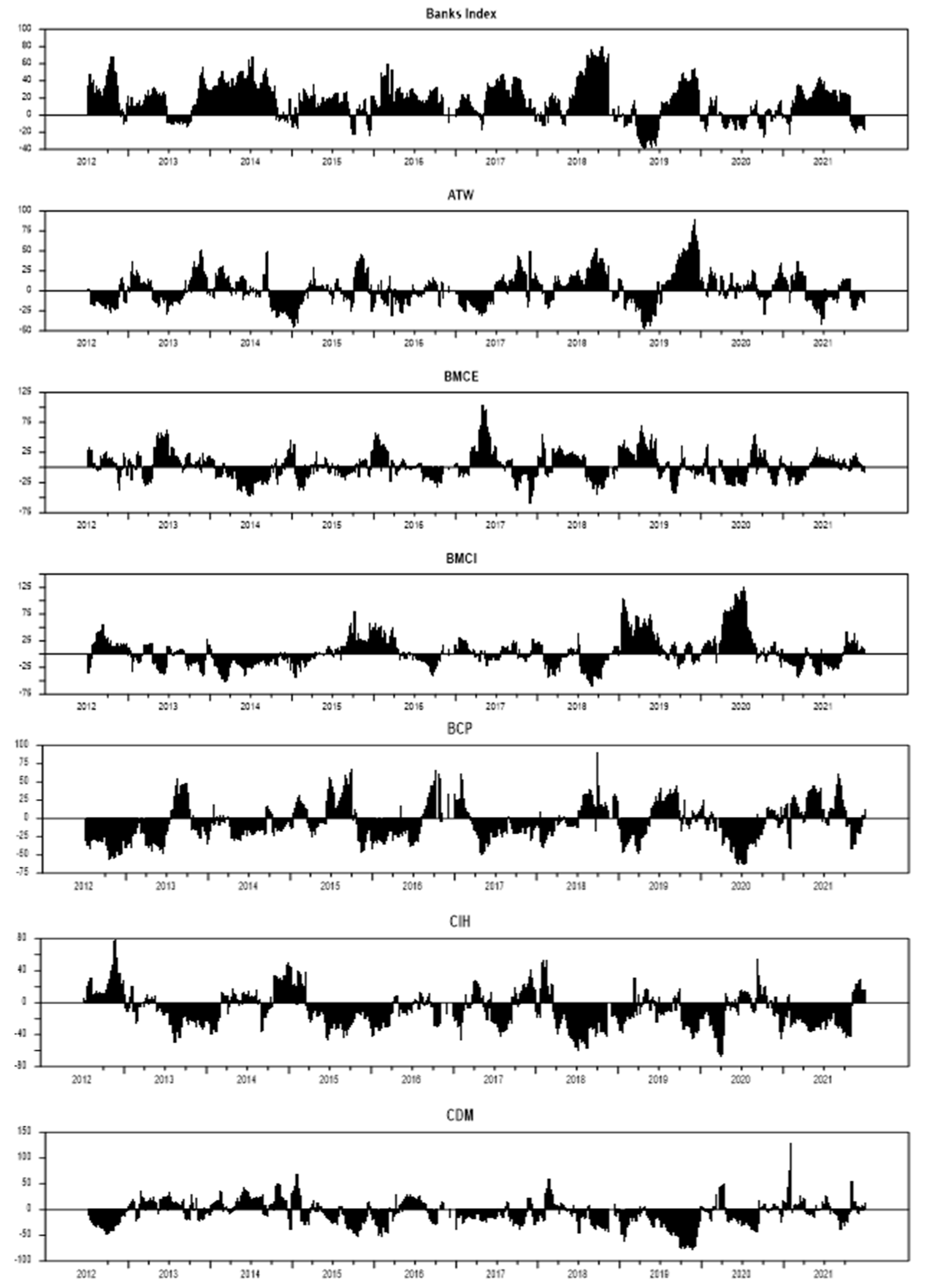
Figure 3 and Figure 4 display the evolution of the daily log returns of the bank index and the six financial institutions before and during the COVID-19 health crisis, respectively.

Table 2. Descriptive statistics and stationarity results (before the COVID-19 crisis).

Before Crisis	BANKS INDEX	ATW	BMCE	BMCI	BCP	CIH	CDM
Mean	0.000095	0.000158	−0.000054	−0.000094	0.000168	0.000062	−0.00026
Median	0.0000375	0	0	0	0	0	0
Maximum	0.038563	0.04512	0.095037	0.095191	0.066273	0.09531	0.094856
Minimum	−0.033636	−0.0501	−0.0835	−0.10096	−0.09706	−0.07841	−0.10528
Std. Dev.	0.007109	0.010261	0.013211	0.021749	0.01028	0.018819	0.02038
Skewness	0.285814	0.178666	0.371141	−0.09192	−0.02052	0.054067	−0.25119
Kurtosis	5.466875	5.447024	9.693836	6.621677	12.21747	5.19444	7.42255
Normality test: Jarque– BeraProbability	523.6657	499.4417	3704.271	1073.944	6938.677	394.2262	1617.926
	0	0	0	0	0	0	0
Unit root test: ADF Probability	−45.58105	−50.192	−52.2934	−31.0853	−48.9221	−39.1363	−22.494
	0	0	0	0	0	0	0

and

Table 3. Descriptive statistics and stationarity results (during COVID-19 crisis).

During Crisis	BANKS INDEX	ATW	BMCE	BMCI	BCP	CIH	CDM
Mean	0.000026	0.0000079	−0.000020	−0.000498	0.000041	0.0003	0.000502
Median	0.000646	0	0	0	0	0	0
Maximum	0.065637	0.060433	0.080503	0.094297	0.071744	0.070543	0.095132
Minimum	−0.103011	−0.105230	−0.104332	−0.105281	−0.10513	−0.104933	−0.09531
Std. Dev.	0.011529	0.013703	0.016639	0.018420	0.012708	0.016153	0.015292
Skewness	−2.017844	−1.26736	−0.629172	−0.375028	−1.89044	−0.767847	0.138628
Kurtosis	23.39902	13.38928	8.575254	7.34.434	21.00118	9.045455	11.4270
Normality test: Jarque– BeraProbability	9386.834	2482.609	709.1437	421.1840	7344.744	844.5819	1543.491
	0	0	0	0	0	0	0
Unit root test: ADF Probability	−20.88472	−20.65237	−25.9065	−24.20456	−23.9102	−26.01147	−23.2273
	0	0	0	0	0	0	0

provide a summary of some descriptive statistics of the geometric yield series in the two defined sub-periods. The kurtosis is well above 3 for all series, indicating that the distribution of returns is sharp (leptokurtic). In addition, the Jarque–Berra normality test (p < 0.0001) reveals a statistically significant deviation of the data from the Gaussian distribution. The statistics from the Ljung–Box (1978) test show that the log return series has autocorrelation.

For all financial series of geometric returns, the standard ADF (Augmented Dickey-Fuller) unit root test (1979) was performed, as presented in Table 2 (pre-crisis period) and Table 3 (crisis period). The ADF statistic for all log return series is below their critical values at the 1% significance level. This means that these series do not have unit roots and are not moving, which means they can be used for further analysis.

5. Empirical Results

In this section, we measure the volatility spillovers of returns during the pre-crisis and during-crisis sub-periods for the assets of the five banks and the banking index. The spillover index will allow us, on the one hand, to indicate the connectivity and volatility transmission between each asset pair $\left(i,j\right)$ in both directions ($i\overrightarrow{ to }j and i \overleftarrow{from} j \left(\forall i\ne j\right)$) and between each institution $i$ and all other banks ($i\overrightarrow{ to all }j and i \overleftarrow{from all} j \left(\forall i\ne j\right)$). On the other hand, thanks to this index, we can rank banks according to their systemic importance in the interbank market in terms of the weight of volatility transmissions with the banking sector index.

Here, we present the description of the static spillover index for returns and volatility. In addition, we calculate the average directional spillovers and the average net spillovers before and during the COVID-19 health crisis. This can tell us a lot about how the spillover effect is passed on between the institutions that make up the Moroccan interbank market.

In

Table 4. Volatility spillover index (pre-crisis period).

	Banks Index	ATW	BMCE	BMCI	BCP	CIH	CDM	Contribution from Others
Banks Index	63.61	23.85	3.49	0.18	7.35	1.47	0.04	36.4
ATW	29.32	67.61	0.05	0.03	0.41	2.52	0.06	32.4
BMCE	5.40	0.36	91.76	0.27	1.57	0.5	0.15	8.2
BMCI	0.51	0.36	0.26	96.45	0.35	2.02	0.05	3.6
BCP	10.17	0.79	0.36	1.17	86.72	0.80	1.3	14.6
CIH	2.87	0.89	1.16	0.11	0.23	93.5	1.24	6.5
CDM	1.37	0.67	0.87	0.24	0.57	0.84	95.44	4.56
Contribution to others	49.64	26.92	6.19	2	10.48	8.15	2.84	106.22
Contribution to others including own	113.25	94.53	97.95	98.45	97.2	101.65	98.28	701.31
Spillover net *	13.26	−5.47	−2.06	−1.55	−4.11	1.65	−1.72	SI = 15.14% **

* Spillover net = (contribution to others − contribution from others); ** Spillover index.

and

Table 5. Volatility spillover index (during-crisis period).

	Banks Index	ATW	BMCE	BMCI	BCP	CIH	CDM	Contribution From Others
Banks Index	37.59	23.84	11.21	3.91	19.10	4.28	0.07	62.4
ATW	24.90	43.5	8.32	4.12	14.99	4.03	0.14	56.4
BMCE	7.45	3.48	57.03	6.98	4.90	3.30	17	43.11
BMCI	1.79	2.07	11.77	82.52	0.73	1.03	0.08	17.47
BCP	12.17	9.63	5.31	1.06	58.58	11.11	2.15	41.43
CIH	3.02	4.09	0.15	0.51	4.46	84.76	3.01	15.24
CDM	2.03	0.98	1.04	0.67	2.17	2.04	9.17	8.93
Contribution to others	51.36	44.09	37.8	17.25	46.35	25.79	22.45	245.09
Contribution to others including own	88.95	87.59	94.83	99.77	104.93	110.55	113.62	700.24
Spillover net *	−11.05	−12.41	−5.31	−0.22	4.92	10.55	13.52	SI = 35% **

* Spillover Net = (Contribution To Others − Contribution From Others); ** Spillover index.

, the underlying variance decomposition is the basalized variance decomposition of KPPS. In addition, the ${ij}^{\mathrm{th}}$ entry is the estimated contribution to the variance of bank i’s 10-day forecast error due to shocks from bank j. The first row shows assets from which the spillovers emanate. The first column refers to the assets receiving the spillovers. The column “From Others” shows the sum of spillovers received by the asset listed in the first column. The row “Contribution to Others” is the sum of spillovers from the asset listed in the first row.

The “Net Volatility Spillover” row gives the difference in total directional spillovers (“Contribution to others” minus “From others”). The total spillover index is the sum of all the columns and rows that are not on the diagonal compared to the sum of all the columns and rows that are on the diagonal, given as a percentage.

5.1. Pre-Crisis Sub-Period: From 1 January 2012 to 31 December 2019

Table 4 provides an approximate decomposition of the volatility spillover index before the COVID-19 pandemic crisis.

Analyzing the results in Table 4, we noticed that the gross directional spillovers of the banking sector index are very strong; its “Contribution to others” value amounts to 49.64 percent of the variance of the forecast errors of the volatility of the banks’ geometric returns. On the other hand, its “from others” value is equal to 36.4 percent of the variance of volatility forecast errors. In other words, shocks to the volatilities of the banking sector index are responsible for 49.64% of the variance of the volatility forecast errors of financial institutions, while the index received 36.4% of the volatility shocks from banks.

As for the net spillovers from the banking index, they are equal to 13.26%. This positive value shows that the weight of the transmitted volatility shocks is stronger than the shocks received in the pre-crisis period.

Individually, the gross directional volatility spillovers from the sector index to the other individual banks vary from one bank to another. ATW bank recorded the highest value and amounts to 29.32%. This indicates that 29.32% of ATW bank’s volatility shocks are produced due to market shocks, which puts this bank at the top of the systemic banks sensitive to market shocks. As for BMCI bank, we noticed that the gross directional impact of the stock index on this stock is very low; its value “Contribution BMCI from Banks index” is maintained only at 0.51%, which allows us to classify BMCI bank as the least sensitive bank to market shocks in terms of systemic importance. The other banks (BCP, BMCE, CIH, and CDM) have values close to 10.17, 5.40, and 1.37 for percentage of their contribution to the market, respectively.

The spillover index amounts to 15.14%, which is a key figure of the summary results; it shows that 15.14% of the forecast error variance results from volatility spillovers. Therefore, on average, the spillovers transmitted in the Moroccan interbank system are significantly large, and they reflect a real level of financial connectivity between Moroccan banks.

5.2. During-Crisis Sub-Period: From 1 January 2020 to 31 December 2021

Table 5 presented above provides an approximate decomposition of the volatility spillover index during the COVID-19 pandemic crisis.

During the COVID-19 pandemic crisis, the gross directional spillovers from each market increased significantly. In fact, Table 5 shows that the market is responsible for 51.36 percent of the error in volatility forecasts during the pandemic crisis—up from 49.64 percent before the crisis.

For the “from others” value, it increased from 36.4% (before the crisis) to 62.4% (during the crisis), indicating that the magnitude of the volatility shocks to the banking sector index caused by the six banks’ shocks was strongly impacted by the COVID-19 crisis.

As for the net spillovers of the banking index, it is −11.05%. This negative number shows that the weight of the volatility shocks that are passed on is small compared to the weight of the shocks that are received during a crisis.

During the crisis, the net spillovers of the index went from +13.26% to −11.05%, which is a big change.

This shows that the individual bank spillovers in the market during the crisis were much bigger than those before the crisis.

This change is due to the fact that the effects of the crisis are spreading faster through the interbank system in Morocco.

Over the crisis sub-period, net spillovers to individual banks increased significantly. It is interesting to note that the spillovers from market shocks experienced by the ATW share were apparently much larger than the other banks and represent the main contribution (24.90%), for the CDM bank share, they represents the lowest contribution of 0.07%. The contribution of market spillovers suffered by other banks amount to 12.17% for BCP, 1.79% for BMCI, 7.45% for BMCE, and finally 3.02% for the CIH share.

The spillover index is more important and clearly increased during the crisis; it reached almost 35%, as increased from 15.14% before the crisis. This rise is due to the fact that the effects of the crisis on the assets of the six banks and the market index are becoming stronger.

5.3. Dynamic Spillover Index (before and during COVID-19 Crisis)

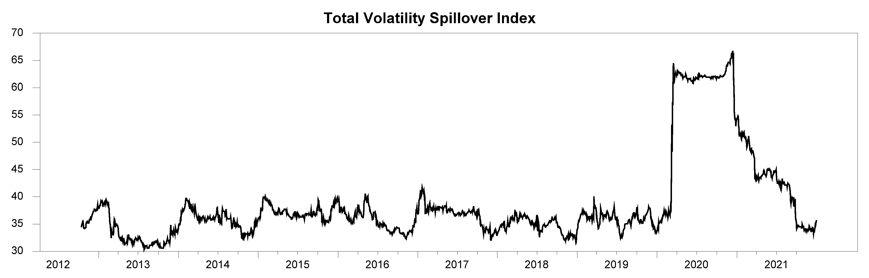
Figure 5 presents the evolution of the conditional volatility of the stocks of the six banks and the banking sector. This remarkable fluctuation in volatility requires a dynamic analysis of the transmission of shocks from this volatility between the different stocks.

After the static analysis of the spillover effect in the Moroccan banking sector, we will therefore move to a dynamic analysis of the rolling sample. Because return volatility and its spillover effects vary over time, a dynamic analysis will make our study more interesting and relevant. We have drawn the volatility spillover curves using 200-day rolling samples and 10-day forecast errors.

5.3.1. Total Volatility Spillover Index

In Figure 6, starting from a value slightly above 30 percent at the end of 2012, the volatility spillover index generally shows a dynamic movement and exhibits a slight trend, sometimes up and sometimes down, varying between 30 and 40 percent until the beginning of 2020, when this index presented a dramatic increase, reaching values close to 65 percent.

The high volatility spillover values observed in Figure 6 during 2020 characterize the COVID-19 pandemic crisis and its consequences for the Moroccan economy in general and the financial market in particular.

During the year 2020, from a value slightly above 35% at the end of 2019, the spillover volatility graph recorded a very sharp increase in its value where it reached almost 65%; it then fluctuated between 60% and 70%, especially from early 2020 to early 2021. During the year 2021, after a gradual decline, the spillover index reached values close to 35%—identical to the levels reached before the year 2020.

5.3.2. Total Directional Spillover

We will subsequently present a dynamic analysis using sliding estimation windows of total directional connectivity for each action.

We will focus on the dynamics of directional connectivity over time.

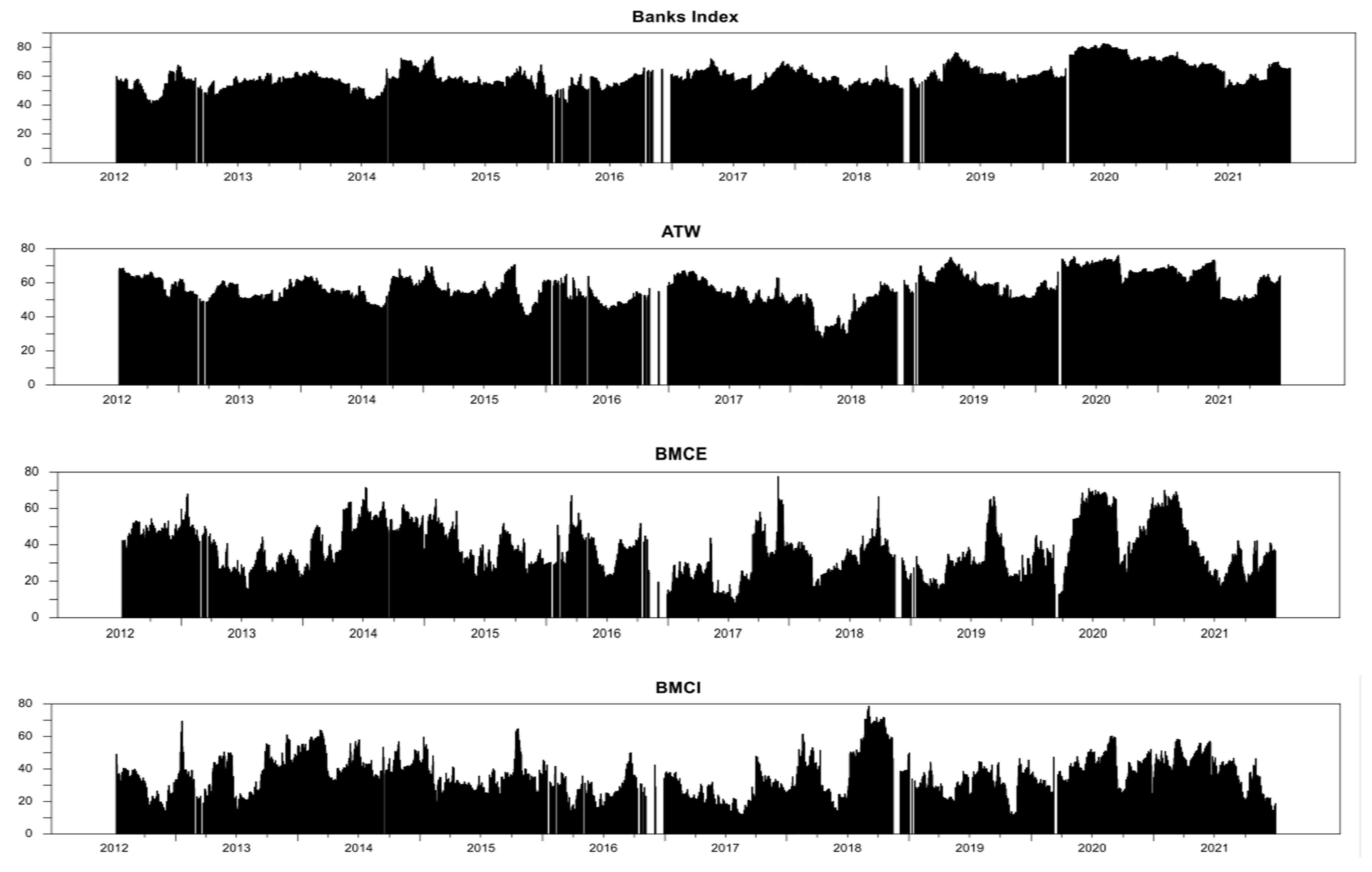
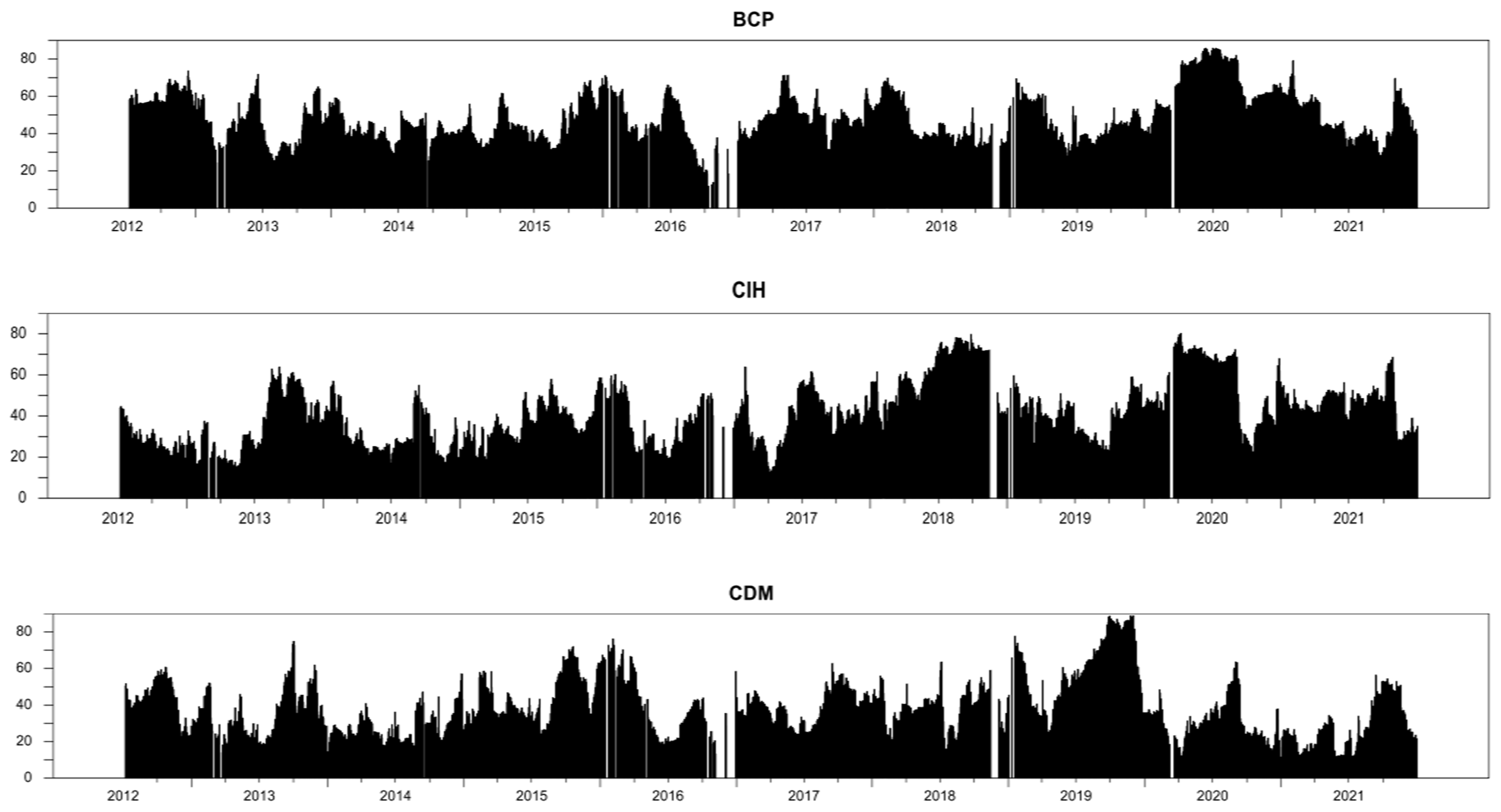
Figure 7 and Figure 8 show the time series of total directional connectivity (“To others” and “From others”) for each bank. Figure 7 shows the plots for the “To others” total direction connectivity curves.

The total directional connectivity curves “From others” are presented in Figure 8, and finally, the total directional connectivity curves “Net” to others are presented in Figure 9.

The first thing to notice in Figure 7 and Figure 8 is the substantial difference between the “to” and “from” plots: the “to others” and “from others” directional spillover curves do not have the same trend or magnitude. The “from others” curves are much smoother than the “to others” curves.

Since the actions of individual institutions are subject to idiosyncratic shocks, some of these shocks may be transmitted to other actions. Some of these shocks are very small and negligible; when a bank that has received a volatility shock, it is possible that this volatility shock will have an even larger contagion effect on the actions of other banks.

In Figure 7, we can see that the “from others” connectivity curves for each stock change and sometimes go up during the sample period. However, the “from” connectivity measures in Figure 7 do not change as much as the “to others” spillover curve in Figure 8.

Both the average “to” and “from” bidirectional connectivity measures are equivalent to the total connectivity measure shown in Figure 6. Each bank has a different bidirectional connectivity to the other banks. As stated, the change in connectivity “from” is much smaller than the change in connectivity “to”.

By analyzing the variation of the net spillover of volatility presented in Figure 9, we noticed that the banking index has almost all positive net spillover values except for a few periods, which shows that the index transmits shocks that have a higher weight than the shocks received by the banks most of the time. The same remark can be made for the BMCI shares. The other banks have net spillovers in most cases—more negative ones than positive ones.

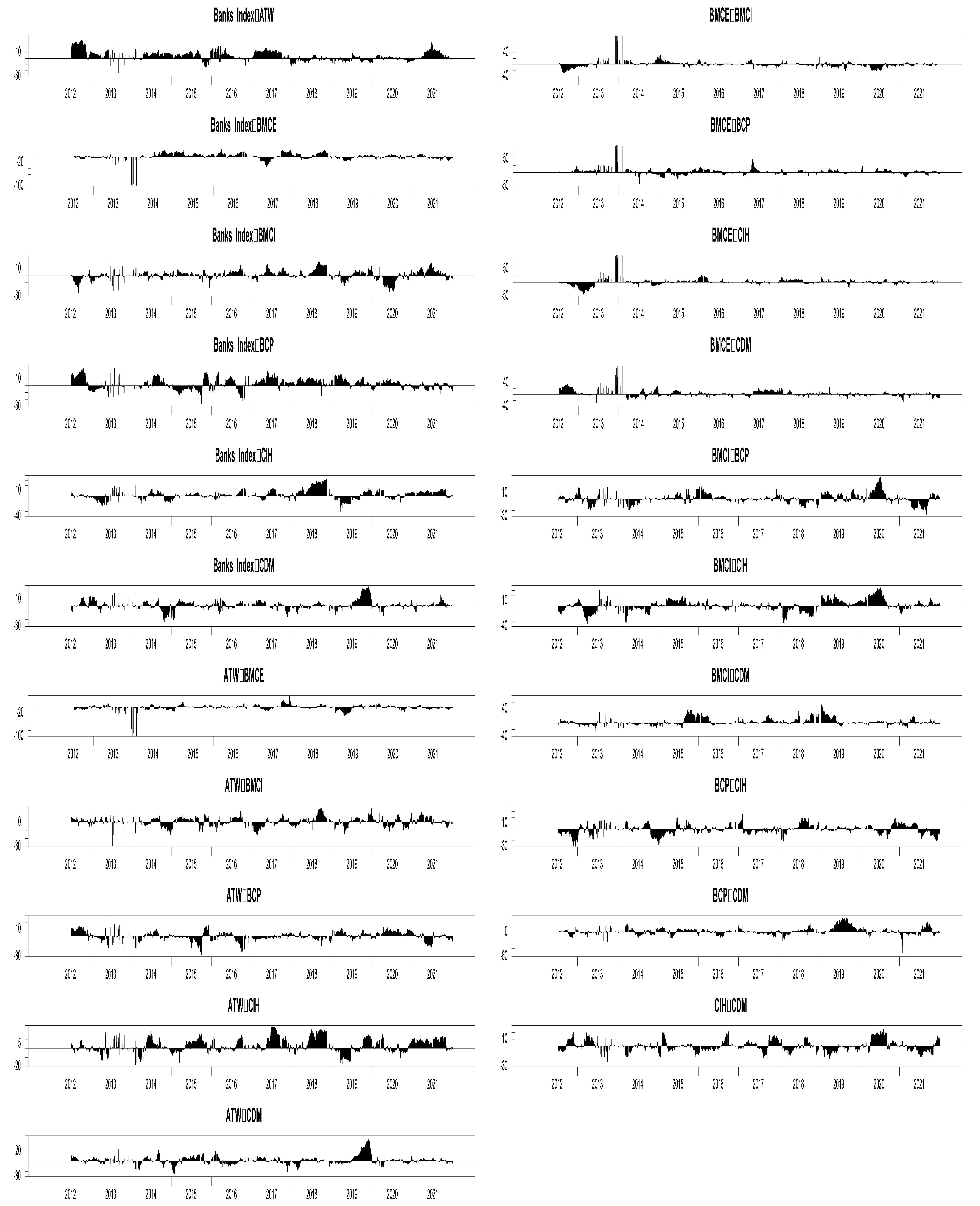
5.3.3. Total Directional Spillover Pairwise

The analysis of pairwise volatility connectivity is important in the analysis of financial contagion. Thus, the importance of pairwise connectivity as a measure of volatility shock transmission between bank stocks and the banking sector stock index should be emphasized. The relevance of pairwise connectedness measures is reflected in the rolling sample windows. The volatility of each financial institution can be affected by the volatility of other institutions, so it is important to look at how pairs of stocks are connected in terms of volatility.

Since there are seven stocks (bank index and six banks) in our sample from 2012 to 2021, it is therefore necessary to present graphs of the volatility connectivity for each of the 21 pairs ($C_7^2$) to analyze how these shocks led to the dynamic volatility connectivity between the stock pairs from 2012 to 2021.

By analyzing the variation of the net volatility spillovers by the pairs presented in Figure 10, we noticed that the pairs (bank index/individual bank) are almost all positive except for a few periods, which shows that the index transmits volatility shocks to the individual banks of greater magnitude than the shocks received by the banks most of the time. For the pairs (bank i/bank j), the degree of connectivity is low, with small positive or negative values.

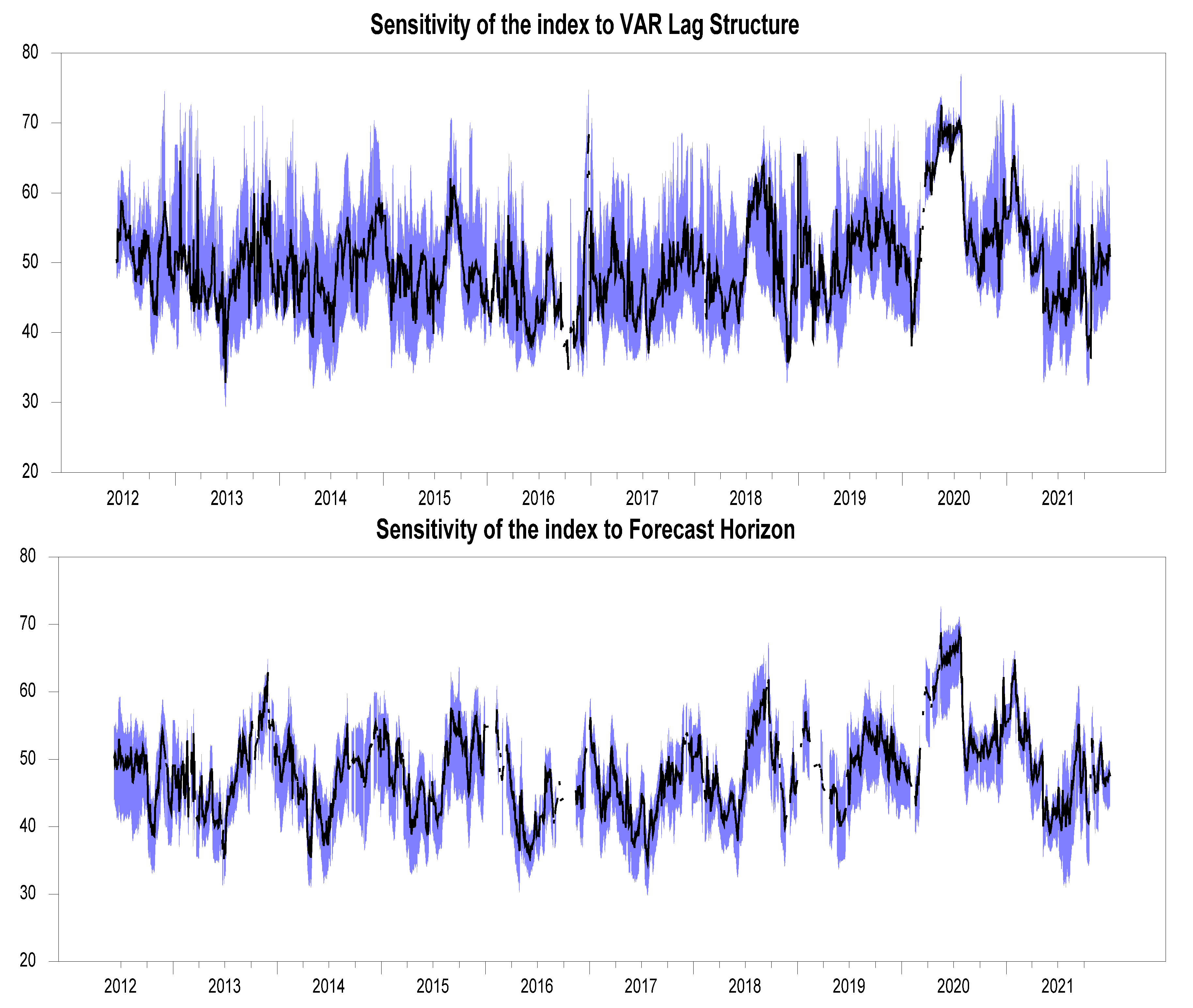
5.3.4. Robustness Assessment of the Total Connectivity

Finally, we conclude this section with an assessment of the robustness of our results regarding the choice of VAR (p) model parameters. We have explored estimation window widths of 200 days and prediction horizons H of 10 days. The black solid line corresponds to our reference order, and the blue band corresponds to an interval (from 10% to 90%) based on 100 randomly chosen orders; the results are presented in Figure 11.

The series evolves very consistently over time, which clearly shows the robustness of our VAR model estimation results regarding either the order p of the VAR model or the time horizon of the sliding window of the dynamic analysis.

It is also important to note that the interval (from 10% to 90%) based on 100 random orders of total connectivity is quite narrow.

6. Conclusions

The banking sector was one of the sectors impacted by the COVID-19 crisis due to the sanitary measures imposed by the pandemic. It is known that a shock in a bank can spread to other banks in the same system, and the failure of a bank can lead to the collapse of the banking system. This collapse of the banking system can be transmitted to the real economy by contagion. Systemic risk can be assessed using several indicators and from several angles.

In this paper, we assess the impact of the COVID-19 pandemic on the Moroccan banking market using a systemic risk quantification approach. This approach collects and analyzes volatility spillovers, which allows the visual and automatic classification of banks according to their contributions to systemic risk.

We used Diebold and Yilmaz (2012, 2014) methods to analyze the impact of the pandemic crisis on volatility spillovers in the Moroccan banking sector, in particular, the banking sector stock index and publicly traded Moroccan banks. Our sample of geometric returns of the stocks of these banks ranges from January 2012 to the end of 2021 (before and during the COVID-19 crisis). We characterized the static and dynamic connectivity of the interbank system using sliding window estimation of the spillover index.

For the static analysis, we found that the connectivity of Moroccan banks’ stocks is strong for the ATW and BCP banks, while the connectivity of the other banks is weak, allowing us to conclude that these two banks are systemic. Dynamically, we found that the connectivity of the banks’ shares and the banking sector index is variable over time, with a sometimes upward and sometimes downward trend with significant spikes. The dynamic spillover index recorded a strong increase during the health crisis COVID-19 in 2020 and then recovered its levels in 2021. During the pandemic crisis, the spillover index went up, which shows that the interbank system in Morocco is now more connected financially.

Our results suggest that regulators can use the metric we used to measure and evaluate systemic events in the financial market as a whole and in the banking sector in particular more accurately.

The results show that contagion among Moroccan banks increased dramatically at the beginning of the COVID-19 epidemic, and that ATW and BCP banks became more systemically important. Finally, these results show that ATW and BCP banks should be given special attention by Moroccan central bank officials because of their high systemic importance.

References

- Adam, Waldemar, Irena Bronstein, Brooks Edwards, Thomas Engel, Dirk Reinhardt, Friedemann W. Schneider, Alexei V. Trofimov, and Rostislav F. Vasil’ev. 1996. Electron exchange luminescence of spiroadamantane-substituted dioxetanes triggered by alkaline phosphatase. Kinetics and elucidation of pH effects. Journal of the American Chemical Society 118: 10400–7. [Google Scholar] [CrossRef]
- Baig, Taimur, and Ilan Goldfajn. 1999. Financial market contagion in the Asian crisis. IMF Staff Papers 46: 167–95. [Google Scholar]
- Calvo, Guillermo A., Leonardo Leiderman, and Carmen M. Reinhart. 1996. Inflows of Capital to Developing Countries in the 1990s. Journal of Economic Perspectives 10: 123–39. [Google Scholar] [CrossRef] [Green Version]
- Demirer, Mert, Francis X. Diebold, Laura Liu, and Kamil Yilmaz. 2018. Estimating global bank network connectedness. Journal of Applied Econometrics 33: 1–15. [Google Scholar] [CrossRef]
- Diebold, Francis X., and Kamil Yilmaz. 2009. Measuring financial asset return and volatility spillovers, with application to global equity markets. The Economic Journal 119: 158–71. [Google Scholar] [CrossRef] [Green Version]
- Diebold, Francis X., and Kamil Yilmaz. 2012. Better to give than to receive: Predictive directional measurement of volatility spillovers. International Journal of Forecasting 28: 57–66. [Google Scholar] [CrossRef] [Green Version]
- Diebold, Francis X., and Kamil Yilmaz. 2014. On the network topology of variance decompositions: Measuring the connectedness of financial firms. Journal of Econometrics 182: 119–34. [Google Scholar] [CrossRef] [Green Version]
- Edwards, Sebastian, and Raul Susmel. 2001. Volatility dependence and contagion in emerging equity markets. Journal of Development Economics 66: 505–32. [Google Scholar] [CrossRef] [Green Version]
- Engle, Robert. 2002. Dynamic conditional correlation: A simple class of multivariate generalized autoregressive conditional heteroskedasticity models. Journal of Business & Economic Statistics 20: 339–50. [Google Scholar]
- Engle, Robert F., and Kenneth F. Kroner. 1995. Multivariate simultaneous generalized ARCH. Econometric theory 11: 122–50. [Google Scholar] [CrossRef]
- Engle, Robert F., and Kevin Sheppard. 2001. Theoretical and Empirical Properties of Dynamic Conditional Correlation Multivariate GARCH. Cambridge: NBER. [Google Scholar]
- Forbes, Kristin, and Roberto Rigobon. 2001. Measuring contagion: Conceptual and empirical issues. In International Financial Contagion. Boston: Springer, pp. 43–66. [Google Scholar]
- Francq, Christian, and Jean-Michel Zakoïan. 2010. Inconsistency of the MLE and inference based on weighted LS for LARCH models. Journal of Econometrics 159: 151–65. [Google Scholar] [CrossRef] [Green Version]
- Garman, Mark B., and Michael J. Klass. 1980. On the estimation of security price volatilities from historical data. Journal of Business 53: 67–78. [Google Scholar] [CrossRef]
- King, Mervyn A., and Sushil Wadhwani. 1990. Transmission of volatility between stock markets. The Review of Financial Studies 3: 5–33. [Google Scholar] [CrossRef]
- Moradi, Mahdi, Andrea Appolloni, Grzegorz Zimon, Hossein Tarighi, and Maede Kamali. 2021. Macroeconomic Factors and Stock Price Crash Risk: Do Managers Withhold Bad News in the Crisis-Ridden Iran Market? Sustainability 13: 3688. [Google Scholar] [CrossRef]
- Parkinson, Michael. 1980. The extreme value method for estimating the variance of the rate of return. Journal of Business 53: 61–65. [Google Scholar] [CrossRef]
- Sadowski, Adam, Zbigniew Galar, Robert Walasek, Grzegorz Zimon, and Per Engelseth. 2021. Big data insight on global mobility during the COVID-19 pandemic lockdown. Journal of Big Data 8: 78. [Google Scholar] [CrossRef] [PubMed]
- Shahzad, Khurram, Taimoor Hassan Farooq, Buhari Doğan, Li Zhong Hu, and Umer Shahzad. 2021. Does environmental quality and weather induce COVID-19: Case study of Istanbul, Turkey. Environmental Forensics, 1–12. [Google Scholar] [CrossRef]
- Yilmaz, Kamil. 2010. Return and volatility spillovers among the East Asian equity markets. Journal of Asian Economics 21: 304–13. [Google Scholar] [CrossRef] [Green Version]
Figure 1.
Evolution of the bank index price before and during the COVID-19 crisis.
Figure 2.
Evolution of bank share prices before and during the COVID-19 crisis.
Figure 3.
Daily return of the bank index before and during the COVID-19 crisis.
Figure 4.
Daily returns on bank shares before and during the COVID-19 crisis.
Figure 5.
Daily Bank Volatility Index Percent.