
Optimal Neural Network Model for Short-Term Prediction of Confirmed Cases in the COVID-19 Pandemic


1
Faculty of Electronic Engineering, University of Niš, Aleksandra Medvedeva 14, 18000 Niš, Serbia
2
Faculty of Civil Engineering and Architecture, University of Niš, Aleksandra Medvedeva 14, 18000 Niš, Serbia
*
Author to whom correspondence should be addressed.
Mathematics 2022, 10(20), 3804; https://doi.org/10.3390/math10203804
Submission received: 1 September 2022
/
Revised: 28 September 2022
/
Accepted: 10 October 2022
/
Published: 15 October 2022
(This article belongs to the Special Issue Artificial Intelligence and Mathematical Methods)
Abstract
:COVID-19 is one of the largest issues that humanity still has to cope with and has an impact on the daily lives of billions of people. Researchers from all around the world have made various attempts to establish accurate mathematical models of COVID-19 spread. In many branches of science, it is difficult to make accurate predictions about short time series with extremely irregular behavior. Artificial neural networks (ANNs) have lately been extensively used for such applications. Although ANNs may mimic the nonlinear behavior of short time series, they frequently struggle to handle all turbulences. Alternative methods must be used as a result. In order to reduce errors and boost forecasting confidence, a novel methodology that combines Time Delay Neural Networks is suggested in this work. Six separate datasets are used for its validation showing the number of confirmed daily COVID-19 infections in 2021 for six world countries. It is demonstrated that the method may greatly improve the individual networks’ forecasting accuracy independent of their topologies, which broadens the applicability of the approach. A series of additional predictive experiments involving state-of-the-art Extreme Learning Machine modeling were performed to quantitatively compare the accuracy of the proposed methodology with that of similar methodologies. It is shown that the forecasting accuracy of the system outperforms ELM modeling and is in the range of other state-of-the art solutions.
Keywords:
COVID-19; artificial neural networks; short-term prediction; time delay neural networks; extreme learning machineMSC:
68T07; 68T201. Introduction
COVID-19, a global pandemic, expressed its initial wave of infection in China’s Wuhan area [1]. It began on December 19th and, according to the World Health Organization (WHO), its expansion is still a large source of concern. All suggested preventative and control mechanisms continue to have limited impact on preventing or slowing the spread of the virus across the world (isolation, detection tests and prophylactic measures). Since its initial report, until the 24th of August 2022, almost 600 million individuals have been infected, while nearly 6.5 million people have died as a result of infection by the virus, making it one of the deadliest in history [2]. The basic and most crucial feature concerning COVID-19 is that it is spreading fast via human-to-human transmission, while the symptoms of COVID-19 can range from fatal to undetectable (around 20% of infected people, especially children). Other significant elements of the COVID-19 pandemic include a high infection rate, variable incubation periods, patients being contagious throughout the incubation period, and symptomatic illness [3,4]. The elderly and those with weakened immune systems, as well as people with special health conditions, are more vulnerable to the serious effects of this pandemic [5,6]. Given the severity and extent of the epidemic, we may infer that a worldwide pandemic, such as COVID-19, has a critical impact on population health, social-cultural activities, and economic development.
As a result, to offer proper and timely health care, it is critical to estimate the severity of the event and identify the number of cases prior to the event [7]. Efficient healthcare system planning is vital for providing prompt and precise treatment to persons suffering from COVID-19 symptoms. Consequently, models for predicting the course of events during a pandemic are required. Many researches have been published in the literature to anticipate the propagation of the COVID-19 outbreak using various mathematical models.
The use of machine learning techniques for projecting COVID-19 infections is a challenging and actual, but also relatively new scientific task. Many researches and results have been conducted and reported since 2019. In [8], both traditional statistical time series analysis approaches as well as new, machine learning forecasting approaches using Recurrent Neural Networks have been employed. The findings imply that the logistic growth model best describes the pandemic’s behavior, that there is sufficient correlation between climatic and movement factors and illness numbers, and that the Long Short-Term Memory (LSTM) network may be successfully used to forecast daily cases. A similar comparison of forecasting methodologies for the same task was performed in [9]. The classical methods of mathematical modeling in this case showed some weaknesses. As the solution to the problem, a new forecasting neural topology in the form of a Recurrent Neural Network with two layers of LSTM blocks and a 1-D Convolutional Neural Network (CNN) was constructed and trained. The neural network-based approach outperformed the traditional mathematical methodology, again. Another study proposed the application of a CNN and temporal Component Transformation (CT) called CNN–CT for the COVID-19 prediction in the US, Mexico, Brazil, and Colombia [10]. Further transformation of the structure implies adjustments of the predictions made by CNN using Autoregressive Integrated Moving Average (ARIMA) and Exponential Smoothing (ES) methods. Such hybrid methodology achieves competitive results with similar state-of-the-art forecasting methodologies. For COVID-19 spread time series forecasting, another popular neural network topology is the multilayer Perceptron, a feedforward type of architecture that is based on the Perceptron neuron model [11]. In this research, it was expected that the neural network learns to predict 6 days later from 20 days of contextualization. This was achieved after the execution of many structural variations in the suggested topology.
Many mathematical methods for predicting the future often become inaccurate or incorrect when analyzed parameters during forecasting of a certain variable are not well known or understood. Sometimes, there is simply insufficient data on everything that influences the predicted variable. If a specific hypothesis is set incorrectly due to bad assessment, i.e., human error, the forecast will be incorrect. Although predicting is based on past occurrences, no one can ensure that history will repeat itself in the same way every time [12]. Sometimes, the key reason for the limitation of the ANN based learning i.e., low accuracy is the random initialization of the network, and the applications of some preselected neural structures with a fixed number of neurons in the network’s layers. Some alternative approaches that could offer more accurate models for solving many forecasting tasks, such as specific neural-like structures based on the Successive Geometric Data Transformations (SGTM), could be used [13,14]. With this new concept of artificial intelligence, both unsupervised and supervised trainings of the neural-like structures could be conducted, in both cases becoming a non-iterative process [15].
On the other hand, according to studies in the field of COVID-19 prediction using statistical approaches, a basic prediction time of several hundred samples is required to achieve satisfactory prediction accuracy [16,17]. Such time series data is presented as a set of trends, random and seasonal components; these models also have a fairly small number of parameters. Time series with a strong trend and seasonal component can be predicted with a shorter base period [18]. Clearly, the quantity of data available in this situation is sufficient enough to use any other prediction approach [19,20,21], but when we look at a curve illustrating the number of infected patients during one year, we can obviously see that historical values of infected patients are not very helpful when it comes to prediction. As a result, we offer the challenge of predicting the number of infected cases in the following day as a deterministic prediction based on very short time series.
In systems theory, artificial neural network models have emerged as a quick and simple modeling and forecasting tool. Because of its computational efficiency and capacity to characterize an unknown system with a small quantity of data, it is one of the most frequently used prediction models in the literature [22]. The ANN forecasting models have achieved acceptable results in various fields, such as ecology [23], economy [24], industry [25,26], communication [27], and medicine [28].
In our study, we employed an ANN that was modified to forecast the number of infected people on a daily basis. The created model will aid decision-makers, doctors, and medical assistants in preparing and understanding the size of the risk, as well as taking adequate precautions to avoid major leaps. A timely assessment of the risk’s magnitude and the necessary planning can both be supported by forecasting techniques. It will be shown that the created forecasting system can successfully model the trend of time series representing six world countries and their daily new confirmed COVID-19 infection cases. Due to the previous success in using Time Delay Neural Network (TDNN) topologies for short-term time series predictions, we have selected this topology as a basic building block for the construction of a new optimal forecasting system. It will be shown that combined forecasts of individual TDNN, with different numbers of neurons in the hidden layer, produce better forecasts that the individual blocks. This will be confirmed on six different datasets representing COVID-19 spread in the Netherlands, Chile, Malaysia, Spain, Canada, and South Africa, for the year 2021. According to the well-known forecasting performance measure procedures, it will be shown that this kind of individual forecasts’ manipulation, can significantly improve forecasting accuracy and reliability.
To demonstrate the effectiveness of the suggested forecasting methodology and to comprehend the benefits of its employing, it was compared to the ELM algorithm, which is an extensively used prediction approach. The same datasets were used for constructing and training the ELM forecasting networks. A number of additional forecasting tests using this cutting-edge approach were carried out in order to create a feeling about the order of accuracy of the proposed methodology. The results of the performance assessments, again, demonstrate higher forecasting accuracy of the optimal TDNN based forecasting methodology compared to the latest state-of-the-art ELM forecasting.
The remainder of this paper is organized as follows. The study areas and corresponding datasets with their properties, as well as the detailed description of the optimal neural network-based forecasting methodology are presented in Section 2. The application of the methodology, its validation, and the analysis of its accuracy for six selected countries and their datasets are discussed in Section 3. The paper ends with the concluding section and ideas for future work.
2. Materials and Methods
2.1. Study Area and Data
Six countries will be the focus of the study and the validation of the new forecasting approach. They are the Netherlands, Chile, Malaysia, Spain, Canada, and South Africa [29]. As can be noticed, these countries differ in a variety of ways that one may find to be correlated with the magnitude of the daily COVID-19 spread. As seen in Figure 1, they are distributed throughout many continents, have various characteristics, including diverse religions [30], socio-political aspects [31], economic and medical developments [32], climatic variations [33], population, and density and territorial sizes [34], etc.
Databases used for this research represent the daily confirmed cases of COVID-19 infections for the selected countries. This parameter was regularly reported for each country over different media and is highly important for the societies and all their systems. They are available at the internet platform of the World Health Organization [35] and are systematically updated. Each dataset comprises of 365 samples corresponding to the new daily confirmed cases for the year 2021. These time series are graphically represented in Figure 2.
In order to display the variability of COVID-19 spread for six different countries, Table 1, with the descriptive statistics of the corresponding dataset is given next.
Brief informative coefficients known as descriptive statistics are used to assess a particular dataset, which may be a sample of a population or a representation of the complete population [36]. Measures of central tendency, measures of variability, and measures of distribution are three types of descriptive statistics. The distribution of values, expressed as percentages or numbers, summarizes the frequency of each possible value of the variable. Measures of central tendency calculate the average or center of a dataset using one of three methods: mean, mode, and median. Measures of variability informs how dispersed the samples are. The spread is composed of three components: range, standard deviation, and variance.
As mentioned before, the datasets used throughout this study were acquired from the World Health Organization web platform. They are represented in the form of non-linear time series data pairs, defined with a date, and the non-negative integer value of newly confirmed COVID-19 cases. The data were collected with daily time intervals and could be downloaded in an xlsx file format for the particular time interval. For the observed datasets for the year 2021, with 365 daily samples, the minimal number of new confirmed cases of COVID-19 infections ranged from 259 in South Africa, to 1464 in Spain. The maximal number of new confirmed cases goes from 7321 in Chile up to 88,040 in Spain. According to the descriptive statistics of the datasets, the average number of daily confirmed COVID-19 cases was between 3290 in Chile and 11,340 in Spain. All these counts confirm the significant variation of data and its non-periodicity at the annual level.
2.2. Forecasting Methodogy
Generally, neural network-based computing and forecasting approaches arose from the need to uncover, understand, and imitate the brain’s information-processing capabilities [8]. The entire brain is made up of approximately 86 billion neurons that accept data from the environment, isolate and recombine the most important ones, and make judgments regarding the organism’s requirements. In order to perform complicated nonlinear input-output transformations, artificial neural networks (ANN) replicate such brain capabilities.
A time series is a succession of numerical data that occurs at regular intervals across time and is gathered in a sequential way. Short time series are distinguished by a lack of trend information, unpredictability, and periodicity, which makes their prediction a difficult job. Typically, time series situations with very short sample lengths N are inapplicable for producing statistically accurate forecasting variations. This study will concentrate on such time series and their predictions.
We shall explain a novel way for dealing with irregular series. In time series prediction, the neural network topology for a specific task involves determining the number of layers and total number of nodes in each layer. Because there is no theoretical foundation for establishing these characteristics, they are normally established by experimenting with the available data. It has been demonstrated that neural networks with one hidden layer can approximate any nonlinear function with the appropriate number of nodes in the hidden layer, and a suitable dataset for training [37,38,39]. Estimating the number of input nodes that are delayed observations of the same variable is important in time series analysis because it aids in understanding the autocorrelation structure of the data. The number of output nodes may be calculated quite easily. In this work, the Box-Jenkins method’s iterative technique is applied to perform multistep forward forecasting utilizing one output node. The anticipation of the future value includes using the predicted value as an input. It is usually preferable to choose a model with few hidden layer nodes since it performs better at out-of-sample forecasting and does not have fitting issues. The neural network topology cell used throughout this study represents a variant of a Time Delay Neural Network [37,40]. This basic neural network cell (Time Delay Neural Network Cell—TDNNC) is used as a building block for modeling an optimal short-term forecasting neural system. This concept may be used for various types and topologies of neural networks, as well as for comparable AI-based forecasting systems, to increase their accuracy.
TDNN is the type of neural configuration similar to feedforward neural networks, except that the discretized input signals are shifted in time using delay elements, and they are forwarded to the input layer of neurons. Because of that, time series data are suitable for inputs, since they represent a set of samples or measurements of an unknown function f(t) that were gathered over time at regular intervals ∆t. This network has only one output, which is sufficient for one-step-ahead prediction and for the implementation of some kind of dynamic short-term memory.
As mentioned before, a time series: (ti, yi), i = 1, 2,..., N (N is the number of available samples) is a collection of observables of an unknown function ŷ = f(t) collected at regular time intervals ∆t, where ti+1 = ti + ∆t. Data collected in the past are utilized to estimate the future trends of the observed variable during the forecasting process. In order to enable one-step-ahead predictions, it is necessary to find the optimal mathematical form of the function f(t) that can correctly carry out the following transformation:
where ε denotes the acceptable forecasting error, while ŷ(i + 1) is the desired output value.
y(I + 1) = f(ti+1) = ŷ(I + 1) + ε,
The development of ANNs as a tool with remarkable capabilities for identifying and modeling patterns of time series data that are difficult to identify by conventional statistical approaches has taken place during the past few decades. However, there is one aspect that most current ANN implementations for prediction share. In order to reach high prediction accuracy, a rather large time series is required. Typically, there have to be at least 50 data points to take into account [41]. However, the general opinion is that data from the recent past are more important than older ones and should have a significantly greater impact on the final prediction result. Based on this, we conclude that even in the case where we have a long time series at our disposal, we should apply methods that rely on short series. This, together with other studies that we have conducted in short-term forecasting [42,43,44], were the reasons that led us to select the Time Delay Neural Network architecture as the foundation for this research. A structure of a basic TDNNC is shown in Figure 3 and will be briefly explained next.
The topology requires a neural network with one input, which is then delayed and delivered to the input layer neurons. For this purpose, after experimenting with a different number of delay blocks, it was decided to use nine previous observations for the neural network training and prediction, and accordingly nine neurons in the input layer. The hidden layer neurons are activated by the sigmoid activation (logistic) function. Finally, the neurons in the output layer have a linear activation function, and since the aim is to perform one-step-ahead prediction, only one output of the network and, accordingly, only one neuron in the output layer is sufficient for the task. During the ANN training, a variation of the steepest-descent minimization algorithm is used [45,46,47].
A generalized form for obtaining the TDNNC output signal, i.e., prediction in the next time instant is given by:
where and represent the activation functions at the output and hidden layer, respectively, h denominates the number of the neurons in the hidden layer, represents the weight function (sigmoid shape) between the i-th neuron in the input layer and the j-th neuron in the hidden layer, and finally, denominates the weight function (linear function) between the j-th neuron in the hidden layer and the neuron in the output layer. Threshold values for the neurons in the hidden layer and one for the output layer are denoted with and , respectively. As shown in Figure 3, there are always 9 neurons in the input layer, while the number of neurons in the hidden layer can vary from 3 to 10. For the initialization of the network parameters, the methodology in [48,49,50] was used.
The quantity of valuable information in the data and its quality are important elements in determining how well a machine learning algorithm can learn. As a result, it is vital that we inspect and preprocess a dataset before feeding it to a learning algorithm [51]. This facilitates mathematical calculations during the training and forecasting process. It implies shifting, normalizing, and smoothing the pairs of data [15]. In the case of our COVID-19 prediction, the time variable and corresponding response had to be transformed using the following Equation (2):
Here, stands for a constant time instant that reduces the time variables in order to have value 1 for as the first sample in the dataset, value 2 for the second sample, etc. Equation (3) gives the transformation of the response y:
where represents the current instance of the target function, while M represents a constant, which could be used to reduce the relative difference between the response values, if necessary. It should be noted that the available datasets were already accommodated when acquired. All six time series sets have no extreme jumps, no negative values, no trend, and no seasonality. During the data acquisition, it was possible to select an option 7-day-moving-average, which further smoothed the fluctuation of the data trend in the 7-days’ time window, which is especially important when dealing with the data collected for the non-working days and weekends. The corresponding formula for a simple moving average procedure (SMA) is given as (5):
In this equation, , …, represent the values of the target function from the N-days wide time slot.
When analyzing the architecture shown in Figure 3, it should be emphasized that the main idea for developing and using this structure is to force the network to learn the same input-output mapping several times through several shifts in time. In this way, it is supposed that the previous samples of data will have a larger influence on the future outcomes. At the same time, the network captures complex intricately entwined deterministic relationships that influence the occurrences and trends of the observed variable. When dealing with a univariate time series dataset, the resulting function needs to perform the following transformation:
where represents the error of the prediction at the time t + 1, i.e., the difference between the expected value at that time and the value that the network obtains.
The aim of the training is to minimize the predicting error by optimizing the network parameters. After the training, the TDNNC will perform an approximation of the function that represents the given time series and will also be able to extrapolate the values outside the time interval, i.e., to forecast.
Figure 4 depicts the methodology for improving the accuracy and certainty of the short time series ANN prediction that we propose. The purpose of this research is to create tools and procedures that will improve the accuracy of many existing individual forecasting TDNNC blocks while simultaneously utilizing the best of them.
We start with a short time series (only nine samples) that expresses one variable over a short period of time and that can be properly accommodated in order to facilitate their learning. The accuracies of forecasts are then assessed as a result of altering the number of neurons in the hidden layer of the single TDNNC. Eight different TDNNCs are built and trained using the same datasets, starting with one that has three neurons in the hidden layer and ending with one that has ten neurons in the hidden layer.
When a set of eight TDNNCs is trained, as mentioned before, this requires a learning set of nine samples (in our case, this is shown to be enough) in order to create the first forecast at their outputs, that is, the extrapolated values of their trend functions. We also calculate the first forecasting error for the particular network. Now, we shift the learning set of nine samples for one time step and repeat the training process. By entering every further sample set at the input, the networks better learn and predict the trend and its change. As already mentioned, this process repeats for the entire group of eight networks for each time step of the entire time series.
Since each dataset is very small, and the TDNNCs are very simple, each forecasted value requires a minimal amount of time and mathematical effort to be completed.
At the end of this process, all networks are trained with the entire time series dataset. The output of this procedure can be systematized as a forecasting matrix, in which rows correspond to the time instances for which the forecasts were produced, while the columns correspond to the number of hidden neurons in a specific TDNNC. There are eight columns in the forecasting matrix.
We introduce the forecast of the full group of TDNNCs to boost the confidence of the prediction and its accuracy, since it is impossible to determine which of the eight TDNNCs is more accurate for a specific portion of the entire time series dataset. Specifically, we first exclude two forecasts that represent the minimal and maximal predicted values out of the eight forecasts made for the same short time series. In this way, it is the most likely that the worst-case forecasting values that could converge in a wrong direction are discarded from further forecasts. This process leaves us now with six individual forecasted values to deal with. Further improvement implies averaging all of them. The averaged value represents the final forecast of the system. It will be shown that these few manipulations with the individual TDNNC’s forecasts may significantly increase the accuracy of the predictions. In addition, this procedure, despite its dedication to the short time series datasets, by shifting and repeating the procedure, successfully and efficiently deals with a long time series.
2.3. Prediction Accuracy Measures
Root-Mean-Square-Error or RMSE: While training regression or time series models, RMSE is one of the most commonly used metrics to assess the accuracy of the forecasted values of the model vs. the actual or observed values. When the target or response variable is a continuous number, it assesses the inaccuracy in our anticipated values. It shows how far apart the data is from the line of best fit. It is also an important criterion for selecting the best performing model among several forecasting models trained on a same dataset. It can be calculated using Equation (7):
where N represents the number of observations, while yi and ŷi are the obtained and expected value of the forecast, respectively.
Mean Absolute Percentage Error: Another performance measure for the forecasting system that will be used here is the Mean Absolute Percentage Error or MAPE. It shows, on average, how accurate the anticipated quantities were in relation to the actual values by averaging the absolute percentage errors of each entry in a dataset. Larger datasets can typically be more effectively analyzed using MAPE, although zero-valued datasets cannot have their MAPE calculated. The equation for calculating MAPE is given as (8):
Coefficient of determination or R2: This coefficient can range between 0 and 1 and shows how well a forecasting model predicts the outcome. It is a measure of the goodness of fit. Its higher value corresponds to a better prediction for a model. It can be calculated as (9):
where represents the mean of the observed variable.
3. Results and Discussion
The forecasting performance of the suggested methodology is evaluated with datasets recorded for six countries for the year 2021. For each of six countries (Chile, the Netherlands, Spain, Canada, South Africa, and Malaysia), eight different TDNNCs are constructed. After applying training and forecast procedures, we have obtained final forecasts. They are systematized against their corresponding expected values on the graphs shown in Figure 5a–f. Bearing in mind that the characteristics of different sets of data vary from country to country, it can be noticed that the suggested forecasting system performed very well.
In order to confirm the increase in the forecasting accuracy of this system in comparison to the initial individual TDNNC structures, we have calculated the relative percentage forecasting errors for all six countries for eight TDNNC blocks with the number of neurons in the hidden layer ranging from three to ten.
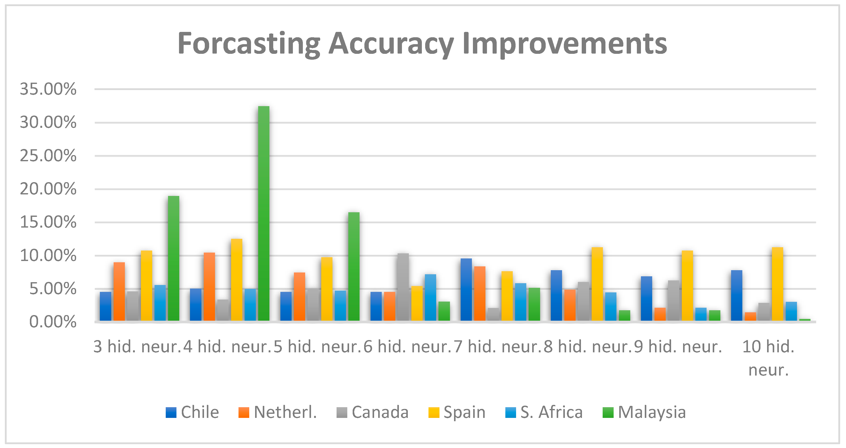
The relative percentual forecasting error for the suggested forecasting system is shown in the first column of Table 2, while the relative, i.e., percentual differences, between the accuracy of the suggested forecasting system and the individual TDNNCs’ forecasts are shown in the remaining eight columns. It can be noticed that the entire system outperforms the individual TDNNCs when observing the forecasting error for the year 2021 and fulfills the expectations. Using the suggested system, the increase in relative accuracy goes from 0.45% in the case of Malaysian TDNNC with 10 hidden neurons, to 32.42% in the case of TDNNC with four hidden neurons. This is also illustrated in Figure 6. Here, the X-axes denote the individual TDNNCs realization, while the Y-axes denote the percentual increase of the forecasting accuracy (relative error) between their individual forecasts and the forecasts of the optimal TDNNC based forecasting system that incorporates several individual TDNNCs. For example, the forecasting accuracy of the system (calculated as the averaged relative error of the forecasts) is larger than the accuracy achieved using only a single TDNNC for the same prediction. These increases are graphically represented with bars in different colors in Figure 6, where each color corresponds to a particular country.
As another measure of performance, we have calculated the RMSE, MAPE and R2 of the system’s forecasts for all six analyzed countries. This is shown in Table 3.
In order to compare the suggested methodology with alternative ones, we have conducted new research and a large number of experiments that employ the Extreme Learning Machine (ELM) algorithm for the same forecasting tasks [2,3,4,5,6,7,8,9,10,11,12,13,14,15,16,17,18,19,20,21,22,23,24,25,26,27,28,29,30,31,32,33,34,35,36,37,38,39,40,41,42,43,44,45,46,47,48,49,50,51,52,53,54]. ELM is a relatively new machine learning paradigm. Among all neural network topologies, this is one of the most efficient ones because its parameters are set only once, and because of the high-speed non-iterative training. Due to its simplicity, this algorithm is easy to understand, implement, and solve complex problems with. However, the proposed optimal TDNNC based prediction method shows a better prediction ability than this state-of-the-art machine learning method. The comparison of the performance measure values for these two methodologies, for six analyzed countries, is also systematized in Table 3. It could be noticed that the suggested methodology outperforms the alternative ELM methodology when considering every type of performance measure.
It was already mentioned that, throughout this study, we have analyzed only one COVID-19 related parameter. That is the number of daily new infections. As shown, these datasets vary in different manners and are very uncorrelated since each country experiences different influences and different types of factors to the number of daily new infections. Because of this, we find that the selected datasets can be used for the verification of the suggested methodology.
When forecasting the daily infections of COVID-19, the results generated using the suggested Time Delay Neural Networks-based methods offer several advantages. In particular, it is extremely unappreciative to utilize mathematical techniques and models to anticipate future trends of infection in various parts of the world. The observed variable is extremely susceptible to turbulence and many different influences. Our system coped well with this problem.
The results in forecasting the new daily COVID-19 infections are of great importance for every country in the world. It can help to estimate the future medical needs of staff, hospital beds, medications, food, money, etc. Because of the inherent characteristics of uncertainty, randomness, and nonlinearity, the COVID-19 cases are still an ongoing world problem. In the case of this forecasting task, we have achieved satisfactory results and different types of forecasting performance measures confirm that. After performing six ELM model accuracy measures’ calculations, the values obtained for RMSE ranged from 1283.14 for Malaysia to 7380.34 for Spain. The MAPE values ranged from 4.66 for Chile to 22.94 for Canada. Finally, the R2 as a measure of goodness of fit ranged from 0.67 for Canada to 0.99 for Chile. The corresponding performance measures in the case of the suggested forecasting methodology performed better than ELM modeling, considering all analyzed types of forecasting errors, as shown in Table 3. For example, the calculated R2 values for our methodology ranged from 0.9896 for Canada to 0.9990 for Malaysia.
Furthermore, in order to evaluate the effectiveness of the proposed methodology, we have conducted a search for some alternative solutions to COVID-19 related prediction problems that are available in the recent literature. These findings for six world countries are systematized in Table 4.
Alternatively, we have analyzed the prediction results and accuracy of new COVID-19 infections in other world regions by applying some alternative neural network approaches. Using a Multi-Layer Perceptron model, with an Extreme Learning Machine learning procedure and different methods of input parameters selection, for predicting COVID-19 in Karnataka State, India, the accuracy reached between 7% and 20%, expressed as the MAPE, and between 29 and 105, expressed as an RMS Error [67]. A classic predictor approach with deep learning architecture using a NAdam training model was described and trained for in a few world countries in [68]. This methodology achieved an accuracy of between 68.7% for the Ontario region in Canada to 100% for the Shanghai, Jilin, and Fujian regions in China. A nonlinear autoregressive neural network time series model has been developed for forecasting COVID-19 cases in [69]. It applies a standard two-layer feed-forward Backpropagation (BP) learning algorithm with sigmoid activation in the hidden layer and linear activation in the output layer and reaches an accuracy of between 0.987 and 1, expressed as the R value. In addition, three deep learning forecasting methodologies for the prediction of COVID-19 confirmations in Australia and the Jordan states were described in [70]. They are the prophet algorithm, ARIMA, and the Long Short-Term Memory (LSTM) neural network. The average accuracy in this study ranged between 88.43% and 94.8%. Considering some Asia-Pacific countries, the latest deep learning techniques were implemented to forecast COVID-19 outbreaks in Pakistan, Afghanistan, India, and Bangladesh [71]. In this study, LSTM, Recurrent Neural Network (RNN), and Gated Recurrent Units (GRU) were applied to quantify the intensity of the pandemic spread in the future. They reach an accuracy of about 90%.
We are aware that the datasets and methodologies that we have analyzed differ from solution to solution, but the most important performance measures, such as MAPE, or the relative percentual forecasting error, of our methodology are in the range of the latest state-of-the-art forecasting COVID-19 methodologies.
4. Conclusions and Future Work
This research proposes a unique way for improving the prediction accuracy of various ANN-based forecasting systems. We provided several effective enhancements for the prediction of short time series by analyzing six separate time series datasets that represent a daily increase in confirmed COVID-19 infections for six countries: Spain, Canada, Malaysia, South Africa, the Netherlands, and Chile. The suggested methodology has been verified on six different datasets. After Time Delay Neural Network blocks models were constructed and trained, their accuracy was assessed using a variety of performance evaluation metrics and statistical tests.
The forecasts of the most accurate individual networks are averaged in a new optimal forecasting system using the highest performing TDNNC topologies, taking into account the number of neurons in the hidden layer. One may conclude that the findings from these case studies related to six worldwide countries show that the average of the six most accurate TDNN individual forecasts could accurately and more confidently predict the trend of future changes, and that the forecast’s accuracy and reliability outperformed those of the individual TDNNC forecasts and even some of the most recent state-of-the-art forecasting techniques, such as the Extreme Learning Machine. Furthermore, we discovered that the accuracy could be improved by up to 32% in the case of Malaysian forecasting. According to the research described in this paper, we may expect the method’s applicability to be expanded to other AI forecasting and modeling methodologies, as well as various types of ANN topologies.
Our future studies will be focused on additional error reductions and the discussion of the least number of neurons in the ANN layers that could accomplish this.
Author Contributions
Conceptualization, M.M. and J.M.; methodology, M.M., J.M. and M.J.; software, J.M. and M.J.; validation, M.M., J.M. and M.J.; formal analysis, M.M. and J.M.; investigation, M.M., J.M. and M.J.; resources, M.M., J.M. and M.J.; data curation, M.M.; writing—original draft preparation, M.M.; writing—review and editing, M.M.; visualization, M.M., J.M. and M.J.; supervision, M.M. All authors have read and agreed to the published version of the manuscript.
Funding
This research was funded by The Ministry of Education, Science and Technological Development of the Republic of Serbia.
Data Availability Statement
The data presented in this study are openly available in https://covid19.who.int, accessed on 24 August 2022.
Conflicts of Interest
The authors declare no conflict of interest.
References
- Wang, C.; Horby, P.W.; Hayden, F.G.; Gao, G.F. A novel corona virus outbreak of global health concern. Lancet 2020, 395, 470–473. [Google Scholar] [CrossRef] [Green Version]
- WHO Coronavirus (COVID-19) Dashboard. Available online: https://covid19.who.int/ (accessed on 15 September 2022).
- Nasserie, T.; Hittle, M.; Goodman, S.N. Assessment of the Frequency and Variety of Persistent Symptoms Among Patients with COVID-19 A Systematic Review. JAMA Netw. Open 2021, 4, e2111417. [Google Scholar] [CrossRef]
- Wang, P.; Lu, J.A.; Jin, Y.; Zhu, M.; Wang, L.; Chen, S. Statistical and network analysis of 1212 COVID-19 patients in Henan, China. Int. J. Infect. Dis. 2020, 95, 391–398. [Google Scholar]
- Gao, Y.D.; Ding, M.; Dong, X.; Zhang, J.J.; Kursat Azkur, A.; Azkur, D.; Gan, H.; Sun, Y.L.; Fu, W.; Li, W.; et al. Risk factors for severe and critically ill COVID-19 patients: A review. Allergy 2021, 76, 428–455. [Google Scholar] [CrossRef]
- Turk, M.A.; Landes, S.D.; Formica, M.K.; Goss, K.D. Intellectual and developmental disability and COVID-19 case-fatality trends: TriNetXanalysis. Disabil. Health J. 2020, 13, 100942. [Google Scholar] [CrossRef] [PubMed]
- Ceylan, Z. Short-term prediction of COVID-19 spread using grey rolling model optimized by particle swarm optimization. Appl. Soft Comput. 2021, 109, 107592. [Google Scholar] [CrossRef] [PubMed]
- Gomez-Cravioto, D.A.; Diaz-Ramos, R.E.; Cantu-Ortiz, F.J.; Ceballos, H.G. Data Analysis and Forecasting of the COVID-19 Spread: A Comparison of Recurrent Neural Networks and Time Series Models. Cogn. Comput. 2021, 1–12. [Google Scholar] [CrossRef]
- Pavlyutin, M.; Samoyavcheva, M.; Kochkarov, R.; Pleshakova, E.; Korchagin, S.; Gataullin, T.; Nikitin, P.; Hidirova, M. COVID-19 Spread Forecasting, Mathematical Methods vs. Machine Learning, Moscow Case. Mathematics 2022, 10, 195. [Google Scholar] [CrossRef]
- Frausto-Solis, J.; Hernández-González, L.J.; González-Barbosa, J.J.; Sánchez-Hernández, J.P.; Román-Rangel, E. Convolutional Neural Network–Component Transformation (CNN–CT) for Confirmed COVID-19 Cases. Math. Comput. Appl. 2021, 26, 29. [Google Scholar] [CrossRef]
- Borghi, P.H.; Zakordonets, O.; Teixeira, J.P. A COVID-19 time series forecasting model based on MLP ANN. Procedia Comput. Sci. 2021, 181, 940–947. [Google Scholar] [CrossRef] [PubMed]
- Milić, M.; Milojković, J.; Marković, I.; Nikolić, P. Concurrent, Performance-Based Methodology for Increasing the Accuracy and Certainty of Short-Term Neural Prediction Systems. Comput. Intell. Neurosci. 2019, 2019, 9323482. [Google Scholar] [CrossRef]
- Shakhovska, N.; Melnykova, N.; Chopiyak, V.; Gregus, M. An ensemble method for medical insurance costs prediction task. Comput. Mater. Contin. 2022, 70, 3969–3984. [Google Scholar] [CrossRef]
- Tkachenko, R.; Izonin, I. Model and principles for the implementation of neural-like structures based of geometric data transformations. In International Conference on Computer Science, Engineering and Education Applications; Springer: Berlin/Heidelberg, Germany, 2018; pp. 578–587. [Google Scholar]
- Tkavhenko, R.; Izonin, I.; Vitynskyi, P.; Lotoshunska, N.; Pavlyuk, O. Development of the Non-Iterative Supervised Learning Predictor Based on the Ito Decomposition and SGTM Neural-Like Structure for Managing Medical Insurance Costs. Data 2018, 3, 46. [Google Scholar] [CrossRef] [Green Version]
- Ahuja, S.; Shelke, N.A.; Singh, P.K. A deep learning framework using CNN and stacked Bi-GRU for COVID-19 predictions in India. Signal Image Video Process 2022, 16, 579–586. [Google Scholar] [CrossRef]
- Al-qaness, M.A.; Fan, H.; Ewees, A.A.; Yousri, D.; Elaziz, M.A. Improved ANFIS model for forecasting Wuhan City Air Quality and analysis COVID-19 lockdown impacts on air quality. Environ. Res. 2021, 194, 110607. [Google Scholar] [CrossRef]
- Polishchuk, E.A. The Analysis of the Selection Criteria of the Optimal Model of the Dynamics in the Case of Extrapolative Forecasting for Short Time Series. In Proceedings of the International Scientific Conference, Far East Con, Online, 17 March 2020; Atlantis Press: Amsterdam, The Netherlands, 2020. [Google Scholar]
- Hernandez-Matamoros, A.; Fujita, H.; Hayashi, T.; Perez-Meana, H. Forecasting of COVID19 per regions using ARIMA models and polynomial functions. Appl. Soft Comput. 2020, 96, 106610. [Google Scholar] [CrossRef] [PubMed]
- Miyama, T.; Jung, S.M.; Hayashi, K.; Anzai, A.; Kinoshita, R.; Kobayashi, T.; Linton, N.M.; Suzuki, A.; Yang, Y.; Yuan, B.; et al. Phenomenological and mechanistic models for predicting early transmission data of COVID-19. Math. Biosci. Eng. 2022, 19, 2043–2055. [Google Scholar] [CrossRef]
- Friston, K.J.; Parr, T.; Zeidman, P.; Razi, A.; Flandin, G.; Daunizeau, J.; Hulme, O.J.; Billig, A.J.; Litvak, V.; Moran, R.J.; et al. Dynamic causal modelling of COVID-19. Welcome Open Res. 2020, 5, 04463. [Google Scholar]
- Tealab, A.; Hefny, H.; Badr, A. Forecasting of nonlinear time series using ANN. Future Comput. Inform. J. 2017, 2, 39–47. [Google Scholar]
- Maier, H.R.; Dandy, G.C. Neural Network Based Modelling of Environmental Variables: A Systematic Approach. Math. Comput. Model. 2001, 33, 669–682. [Google Scholar] [CrossRef]
- Lu, Y.; Mei, G.; Piccialli, F.A. Deep Learning Approach for Predicting Two-Dimensional Soil Consolidation Using Physics-Informed Neural Networks (PINN). Comput. Eng. Financ. Sci. 2022, 10, 05710. [Google Scholar] [CrossRef]
- Qin, Y.; Zhao, M.; Lin, Q.; Li, X.; Ji, J. Data-Driven Building Energy Consumption Prediction Model Based on VMD-SA-DBN. Mathematics 2022, 10, 3058. [Google Scholar] [CrossRef]
- He, L.; Kong, D.; Lei, Z. Research on Vibration Propagation Law and Dynamic Effect of Bench Blasting. Mathematics 2022, 10, 2951. [Google Scholar] [CrossRef]
- Bagnasco, A.; Siri, A.; Aleo, G.; Rocco, G.; Sasso, L. Applying artificial neural networks to predict communication risks in the emergency department. J. Adv. Nurs. 2015, 71, 2293–2304. [Google Scholar] [CrossRef]
- Shahid, N.; Rappon, T.; Berta, W. Applications of artificial neural networks in health care organizational decision-making: A scoping review. PLoS ONE 2019, 14, e0212356. [Google Scholar] [CrossRef]
- World Map. Available online: https://www.mapchart.net/world.html (accessed on 15 September 2022).
- Trepanowski, R.; Drazkowski, D. Cross-National Comparison of Religion as a Predictor of COVID-19 Vaccination Rates. J. Relig. Health 2022, 61, 2198–2211. [Google Scholar] [CrossRef]
- Tang, J.W.; Caniza, M.A.; Dinn, M.; Dwyer, D.E.; Heraud, J.M.; Jennings, L.C.; Kok, J.; Kwok, K.O.; Li, Y.; Loh, T.P.; et al. An exploration of the political, social, economic and cultural factors affecting how different global regions initially reacted to the COVID-19 pandemic. Interface Focus 2022, 12, 20210079. [Google Scholar] [CrossRef]
- Wang, Y.; Yan, Z.; Wang, D.; Yang, M.; Li, Z.; Gong, X.; Wu, D.; Zhai, L.; Zhang, W.; Wang, Y. Prediction and analysis of COVID-19 daily new cases and cumulative cases: Times series forecasting and machine learning models. BMC Infect. Dis. 2022, 22, 495. [Google Scholar] [CrossRef]
- Abu-Abdoun, D.I.; Al-Shihabi, S. Weather Conditions and COVID-19 Cases: Insights from the GCC Countries. Intell. Syst. Appl. 2022, 15, 200093. [Google Scholar] [CrossRef]
- Allain-Dupré, D.; Chatry, I.; Michalun, V.; Moisio, A. OECD Policy Responses Coronavirus (COVID-19), The Territorial Impact of COVID-19: Managing the Crisis across Levels of Government; OECD: Paris, France, 2020.
- Available online: https://worldometer.info/coronavirus (accessed on 15 September 2022).
- Jones, J.S.; Goldring, J. Exploratory and Descriptive Statistics; SAGE Publications Ltd.: London, UK, 2022. [Google Scholar]
- Jha, G.K.; Sinha, K. Time-delay neural networks for time series prediction: An application to the monthly wholesale price of oilseeds in India. Neural Comput. Appl. 2014, 24, 563–571. [Google Scholar] [CrossRef]
- Milojković, J.; Milić, M.; Litovski, V. ANN model for one day ahead Covid-19 prediction. In Proceedings of the Conference IcETRAN, Novi Pazar, Serbia, 6–8 June 2022; pp. 296–300. [Google Scholar]
- Masters, T. Practical Neural Network Recipes in C++; Elsevier: Amsterdam, The Netherlands, 1993. [Google Scholar]
- Yuehjen, E.S.; Lin, S.C. Using a Time Delay Neural Network Approach to Diagnose the Out-of-Control Signals for a Multivariate Normal Process with Variance Shifts. Mathematics 2019, 7, 959. [Google Scholar]
- Zhang, G.; Eddy Patuwo, B.; Hu, Y.M. Forecasting with artificial neural networks. Int. J. Forecast. 1998, 1, 35–62. [Google Scholar] [CrossRef]
- Milojković, J.; Litovski, V. Dynamic Short-Term Forecasting of Electricity Load Using Feed-Forward ANNs. Eng. Intell. Syst. Electr. Eng. Commun. 2009, 17(1), 39–48. [Google Scholar]
- Milojković, J.; Litovski, V. One step ahead prediction in electronics based on limited information. In Proceedings of the Conference ETRAN, Vrnjačka Banja, Serbia, 15–18 June 2019; p. EL1.7. [Google Scholar]
- Milojković, J.; Litovski, V. Short-Term Forecasting of Electricity Load Using Recurrent ANNs. In Proceedings of the Electronics, Banja Luka, Bosnia and Hercegovina, 14 June 2010; pp. 45–49. [Google Scholar]
- Meza, J.C. Steepest descent. In Wiley Interdisciplinary Reviews: Computational Statistics 2.6 2010; Willey: Hoboken, NJ, USA, 2010; pp. 719–722. [Google Scholar]
- Drummond, L.M.G.; Svaiter, B.F. A steepest descent method for vector optimization. J. Comput. Appl. Math. 2005, 175, 395–414. [Google Scholar] [CrossRef] [Green Version]
- Fletcher, R. A limited memory steepest descent method. Math. Program. 2012, 135, 413–436. [Google Scholar] [CrossRef]
- Narkhede, M.V.; Bartakke, P.P.; Sutaone, M.S. A review on weight initialization strategies for neural networks. Artif. Intell. Rev. 2022, 55, 291–322. [Google Scholar] [CrossRef]
- Yam, J.Y.F.; Chow, T.W.S. A weight initialization method for improving training speed in feedforward neural network. Neurocomputing 2000, 30, 219–232. [Google Scholar] [CrossRef]
- Denoeux, T.; Lengelle, R. Initializing backpropagation networks with prototypes. Neural Netw. 1993, 6, 351–363. [Google Scholar] [CrossRef]
- Raschka, S.; Mirjalili, V. Python Machine Learning; Packt Publishing: Birmingham, UK, 2019. [Google Scholar]
- Milić, M.; Milojković, J.; Jeremić, M. A deep learning approach for hydrological time-series prediction with ELM model. In Proceedings of the Small Systems Simulation Symposium, Niš, Serbia, 28 February–2 March 2022; Atlantis Press: Amsterdam, The Netherland, 2022; pp. 61–65. [Google Scholar]
- Das, A.K.; Mishra, D.; Das, K.; Mallick, P.K.; Kumar, S.; Zymbler, M.; El-Sayed, H. Prophesying the Short-Term Dynamics of the Crude Oil Future Price by Adopting the Survival of the Fittest Principle of Improved Grey Optimization and Extreme Learning Machine. Mathematics 2022, 10, 1121. [Google Scholar] [CrossRef]
- Nguyen, D.-T.; Ho, J.-R.; Tung, P.-C.; Lin, C.-K. Prediction of Kerf Width in Laser Cutting of Thin Non-Oriented Electrical Steel Sheets Using Convolutional Neural Network. Mathematics 2021, 9, 2261. [Google Scholar] [CrossRef]
- Díaz-Narváez, V.; San-Martín-Roldán, D.; Calzadilla-Núñez, A.; San-Martín-Roldán, P.; Parody-Muñoz, A.; Robledo-Veloso, G. Which curve provides the best explanation of the growth in confirmed COVID-19 cases in Chile? Rev. Lat.-Am. Enferm. 2020, 28, 1–9. [Google Scholar] [CrossRef] [PubMed]
- Medeiros, M.C.; Street, A.; Valladao, D.; Vasconcelos, G.; Zilberman, E. Short-term COVID-19 forecast for latecomers. Int. J. Forecast. B 2022, 38, 467–488. [Google Scholar] [CrossRef] [PubMed]
- Bekker, R.; Broek, M.; Koole, G. Modeling COVID-19 hospital admissions and occupancy in the Netherlands. Eur. J. Oper. Res. 2023, 304, 207–218. [Google Scholar] [CrossRef]
- Ahterberg, M.A.; Prasse, B.; Ma, L.; Trajanovski, S.; Kitsak, M.; Mieghem, P.V. Comparing the accuracy of several network-based COVID-19 prediction algorithms. Int. J. Forecast. 2022, 38, 489–504. [Google Scholar] [CrossRef]
- Chimmula, V.K.R.; Zhang, L. Time series forecasting of COVID-19 transmission in Canada using LSTM networks. Chaos Solitons Fractals 2020, 135, 109864. [Google Scholar] [CrossRef]
- Zhang, J.; Pathak, H.S.; Snowdon, A.; Greiner, R. Learning models for forecasting hospital resource utilization for COVID-19 patients in Canada. Sci. Rep. 2022, 12, 8751. [Google Scholar] [CrossRef]
- Ahmar, A.S.; del Val, E.B. SutteARIMA: Short-term forecasting method, a case: COVID-19 and stock market in Spain. Sci. Total Environ. 2020, 729, 138883. [Google Scholar] [CrossRef]
- Castillo, O.; Melin, P. Forecasting of COVID-19 time series for countries in the world based on a hybrid approach combining the fractal dimension and fuzzy logic. Chaos Solitons Fractals 2020, 140, 110242. [Google Scholar] [CrossRef]
- Appadu, A.A.; Kelil, A.S.; Tijani, Y.O. Comparison of some forecasting methods for COVID-19. Alex. Eng. J. 2021, 60, 1565–1589. [Google Scholar] [CrossRef]
- Perc, M.; Gorišek Miksić, N.; Slavinec, M.; Stožer, A. Forecasting COVID-19. Front. Phys. 2020, 8, 00127. [Google Scholar] [CrossRef] [Green Version]
- Alsayed, A.; Sadir, H.; Kamil, R.; Sari, H. Prediction of Epidemic Peak and Infected Cases for COVID-19 Disease in Malaysia. Int. J. Environ. Res. Public Health 2020, 17, 4076. [Google Scholar] [CrossRef]
- Salim, N.; Chan, W.H.; Mansor, S.; Bazin, N.E.; Amaran, S.; Faudzi, A.A.; Zainal, A.; Huspi, S.H.; Hooi, E.K.; Shithil, S.M. COVID-19 epidemic in Malaysia: Impact of lockdown on infection dynamics. medRxiv 2020. [Google Scholar] [CrossRef] [Green Version]
- Shetty, R.P.; Pai, P.S. Forecasting of COVID 19 cases in Karnataka state using artificial neural network (ANN). J. Inst. Eng. Ser. B 2021, 102, 1201–1211. [Google Scholar] [CrossRef]
- Wieczorek, M.; Siłka, J.; Woźniak, M. Neural network powered COVID-19 spread forecasting model. Chaos Solitons Fractals 2020, 140, 110203. [Google Scholar] [CrossRef] [PubMed]
- Namasudra, S.; Dhamodharavadhani, S.; Rathipriya, R. Nonlinear neural network based forecasting model for predicting COVID-19 cases. Neur. Proc. Lett. 2021, 1–21. [Google Scholar] [CrossRef]
- Alazab, M.; Awajan, A.; Mesleh, A.; Abraham, A.; Jatana, V.; Alhyari, S. COVID-19 prediction and detection using deep learning. Int. J. Comp. Inf. Syst. Ind. Manag. Appl. 2020, 12, 168–181. [Google Scholar]
- Rauf, H.T.; Lali, M.; Khan, M.A.; Kadry, S.; Alolaiyan, H.; Razaq, A.; Irfan, R. Time series forecasting of COVID-19 transmission in Asia Pacific countries using deep neural networks. Pers. Ubiquitous Comp. 2021, 1–8. [Google Scholar] [CrossRef]
Figure 1.
Study areas: Canada, Spain, the Netherlands, South Africa, Chile, and Malaysia.

Figure 2.
Trends of COVID-19 spread for six world countries in 2021.

Figure 3.
Time Delay Neural Network basic cell.

Figure 4.
Optimal Time Delay Neural Network based Algorithm for Short-Term Prediction.

Figure 5.
Prediction diagrams of COVID-19 daily confirmed infection cases obtained for the year 2021, versus the real daily number of infection cases for (a) Chile, (b) the Netherlands, (c) Canada, (d) Spain, (e) South Africa, and (f) Malaysia.
Figure 5.
Prediction diagrams of COVID-19 daily confirmed infection cases obtained for the year 2021, versus the real daily number of infection cases for (a) Chile, (b) the Netherlands, (c) Canada, (d) Spain, (e) South Africa, and (f) Malaysia.


Figure 6.
Relative forecasting accuracy improvement from individual TDNNC blocks with the number of neurons in the hidden layer varying from three to ten, to the constructed optimal forecasting system, for six world countries.
Figure 6.
Relative forecasting accuracy improvement from individual TDNNC blocks with the number of neurons in the hidden layer varying from three to ten, to the constructed optimal forecasting system, for six world countries.


Table 1.
Descriptive statistics of the COVID-19 daily spread datasets for Chile, the Netherlands, Canada, Spain, South Africa, and Malaysia for 2021.
Table 1.
Descriptive statistics of the COVID-19 daily spread datasets for Chile, the Netherlands, Canada, Spain, South Africa, and Malaysia for 2021.
| Descriptive Statistics | Chile | Netherlands | Canada | Spain | South Africa | Malaysia |
|---|---|---|---|---|---|---|
| Number of scores | 365 | 365 | 365 | 365 | 365 | 365 |
| Mean | 3290.54 | 6348.32 | 4147.86 | 11,340.40 | 6575.88 | 7249.05 |
| Median | 2903 | 4758.5 | 3230 | 7020 | 3514 | 5343 |
| 25th Percentile | 1238.5 | 7493.75 | 2343.5 | 4192 | 1195.25 | 3086 |
| 75th Percentile | 5360.75 | 17,959.25 | 5079 | 15,095.5 | 11488 | 8636.2.5 |
| Interquartile Range | 4122.25 | 4969.25 | 2735.5 | 10,903.5 | 10,292.75 | 5550.25 |
| Minimum | 421 | 588 | 377 | 1464 | 259 | 1211 |
| Maximum | 7321 | 22,471 | 32370 | 88,040 | 23437 | 21,808 |
| Range | 6900 | 32,400 | 31993 | 86,576 | 23178 | 20,597 |
| Variance | 4,951,854.29 | 27,420,731.59 | 13,255,497.17 | 134,112,484.02 | 40,227,254.55 | 35,589,921.39 |
| Standard Deviation | 2225.28 | 5236.48 | 3640.81 | 11,580.69 | 6342.50 | 5965.73 |
| Skew | 0.38 | 1.61 | 3.53 | 2.75 | 0.79 | 1.22 |
| Kurtosis | −1.24 | 2.08 | 19.53 | 11.44 | −0.66 | 0.19 |
Table 2.
Averaged relative error of the entire forecasting system in [%] with the relative accuracy increases achieved using the optimal TDNNC based forecasting methodology in comparison with the individual TDNNCs.
Table 2.
Averaged relative error of the entire forecasting system in [%] with the relative accuracy increases achieved using the optimal TDNNC based forecasting methodology in comparison with the individual TDNNCs.
| Err. of the System | System vs. 3 h. n. TDNNC | System vs. 4 h. n. TDNNC | System vs. 5 h. n. TDNNC | System vs. 6 h. n. TDNNC | System vs. 7 h. n. TDNNC | System vs. 8 h. n. TDNNC | System vs. 9 h. n. TDNNC | System vs. 10 h. n. TDNNC | |
|---|---|---|---|---|---|---|---|---|---|
| Chile | 1.90 | 4.52% | 5.00% | 4.52% | 4.52% | 9.52% | 7.77% | 6.86% | 7.77% |
| Netherl. | 2.75 | 8.94% | 10.42% | 7.41% | 4.52% | 8.33% | 4.84% | 2.13% | 1.45% |
| Canada | 3.75 | 4.58% | 3.35% | 5.06% | 10.29% | 2.09% | 6.01% | 6.25% | 2.85% |
| Spain | 3.16 | 10.73% | 12.46% | 9.71% | 5.39% | 7.6% | 11.23% | 10.73% | 11.23% |
| S. Africa | 3.24 | 5.54% | 4.98% | 4.71% | 7.16% | 5.81% | 4.42% | 2.11% | 2.99% |
| Malaysia | 2.23 | 18.91% | 32.42% | 16.48% | 3.04% | 5.11% | 1.76% | 1.76% | 0.45% |
Table 3.
Performance measures (RMSE, MAPE and R2) for the optimal forecasting system, and for the Extreme Learning Machine forecasting methodology for different countries.
Table 3.
Performance measures (RMSE, MAPE and R2) for the optimal forecasting system, and for the Extreme Learning Machine forecasting methodology for different countries.
| Country | |||||||
|---|---|---|---|---|---|---|---|
| Accuracy Measure | Chile | Netherlands | Canada | Spain | S. Africa | Malaysia | |
| Optimal neural forecasting system | RMSE | 88.67 | 253.80 | 393.74 | 786.68 | 429.43 | 192.30 |
| MAPE [%] | 1.90 | 2.75 | 3.75 | 3.15 | 3.24 | 2.23 | |
| R2 | 0.9984 | 0.9977 | 0.9896 | 0.9955 | 0.9955 | 0.9990 | |
| Extreme Learning Machine | RMSE | 265.46 | 1110.15 | 3134.49 | 7380.34 | 2867.22 | 1283.14 |
| MAPE [%] | 4.66 | 7.8 | 22.94 | 16.68 | 10.77 | 5.69 | |
| R2 | 0.99 | 0.96 | 0.67 | 0.79 | 0.69 | 0.96 | |
Table 4.
Systematization of the current state-of-the-art COVID-19 related forecasting solutions, and their reported performance measures for six analyzed countries.
Table 4.
Systematization of the current state-of-the-art COVID-19 related forecasting solutions, and their reported performance measures for six analyzed countries.
| Country | Methodology | Performance Measure | Ref. | ||
|---|---|---|---|---|---|
| RMSE | Prediction Error [%] | MAPE [%] | |||
| Chile | Different exponential smoothing algorithms | 1.06–1.74 | - | 7.4 | [55] |
| Penalized LASSO regression model with an error correction mechanism | - | - | 0.32–5.22 | [56] | |
| Netherlands | Linear programing method | 5.76–16.15 | - | 5.9–8.2 | [57] |
| NIPA | - | - | 0.04 | [58] | |
| Logistic function | - | - | 0.07 | [58] | |
| Canada | LSTM | 34.83–51.46 | 6.6-7.33 | - | [59] |
| Multiple Temporal Convolutional network | - | 6–9.47 | [60] | ||
| Spain | Sutte ARIMA | - | - | 0.036 | [61] |
| Fuzzy Fractal Approach | - | 3.58139 | - | [62] | |
| S. Africa | Hybrid-Euler | - | 0.56-35.63 | - | [63,64] |
| Malaysia | ANFIS | 46.85 | - | 1.31 | [65] |
| ARIMA | - | - | 16.01 | [66] | |
Publisher’s Note: MDPI stays neutral with regard to jurisdictional claims in published maps and institutional affiliations. |
© 2022 by the authors. Licensee MDPI, Basel, Switzerland. This article is an open access article distributed under the terms and conditions of the Creative Commons Attribution (CC BY) license (https://creativecommons.org/licenses/by/4.0/).
Share and Cite
MDPI and ACS Style
Milić, M.; Milojković, J.; Jeremić, M. Optimal Neural Network Model for Short-Term Prediction of Confirmed Cases in the COVID-19 Pandemic. Mathematics 2022, 10, 3804. https://doi.org/10.3390/math10203804
AMA Style
Milić M, Milojković J, Jeremić M. Optimal Neural Network Model for Short-Term Prediction of Confirmed Cases in the COVID-19 Pandemic. Mathematics. 2022; 10(20):3804. https://doi.org/10.3390/math10203804
Chicago/Turabian StyleMilić, Miljana, Jelena Milojković, and Miljan Jeremić. 2022. "Optimal Neural Network Model for Short-Term Prediction of Confirmed Cases in the COVID-19 Pandemic" Mathematics 10, no. 20: 3804. https://doi.org/10.3390/math10203804
Note that from the first issue of 2016, this journal uses article numbers instead of page numbers. See further details here.