Numerical treatment for a novel crossover mathematical model of the COVID-19 epidemic

1.   Introduction

Despite significant advances in treatment and prevention technologies, contagious diseases continue to impact countless individuals globally. To limit the spread of these diseases, it is imperative to maintain strict control over factors such as transmission routes, population size, rates of human contact, duration of infection, and other critical parameters. Comprehending the behavior and management of pandemic diseases is particularly crucial during the initial infection phases or in the absence of immunization. In this context, mathematical models play an indispensable role. In recent years, scientists from various disciplines have delved into and researched numerous biological models, (see ^[1,2,3] and references therein).

The recent global health crisis, termed the COVID-19 pandemic, stems from the emergence of a novel coronavirus strain, SARS-CoV-2. This virus rapidly evolved into a significant worldwide concern. It has affected millions, placing an unparalleled burden on healthcare infrastructures and economies across the globe ^[4]. In the unyielding fight against this highly contagious and ever-evolving virus, mathematical modeling has proven indispensable. Offering quantitative tools to understand, simulate, and predict the virus's spread, these models have been instrumental in guiding public health measures and shaping policy decisions. Although mathematical modeling has been valuable in past epidemics, its significance has been magnified during the COVID-19 outbreak, where swift and informed decision-making has been crucial^[5,6].

Many systems pertinent to real-world scenarios exhibit crossover behavior. Modeling systems based on this behavior has historically posed significant challenges. The transition from Markovian to non-Markovian processes has unveiled a plethora of examples that highlight real-world complexities. A prime illustration of this is in epidemiology, where the propagation of contagious diseases and occasional chaos may be attributed to this transition. Numerous intricate real-world challenges, including those involving chaos, have been articulated using the frameworks of piecewise integral and differential operators ^[7]. The cited authors delineated three distinct scenarios to frame deterministic-stochastic chaotic models and undertook numerical explorations of these constructs. Additionally, piecewise differentiation has emerged as a potent tool in epidemiological modeling, especially when challenges are presented by crossover dynamics ^[8,9].

Piecewise operators represent a novel class of operators established by Atangana et al. ^[10]. Traditional Mittag-Leffler or exponential mappings in fractional calculus need to provide a precise way to determine crossover time. A unique approach to piecewise derivation addressing this challenge was proposed in ^[10]. Piecewise differential equations offer insights into the present and serve as tools for future planning. Researchers employ these models to simulate diverse scenarios, such as potential virus resurgence and implications of new policy decisions. Active exploration of crossover behaviors with these operators is underway, with studies like ^[11,12] utilizing them to investigate qualitative characteristics of differential equations (DEs) and various infectious disease models. Further applications of piecewise operators are showcased in ^{[13,14,15,16]}.

Atangana et al. ^[9] extended the concept of epidemiology modeling to portray waves with varying patterns, introducing a novel approach to ensure the existence and uniqueness of system solutions. They present a piecewise numerical approach for deriving solutions, with an illustrative example compared against data from Turkey, Spain, and Czechia, concluding that this method offers a new perspective for understanding natural phenomena. Zeb et al. ^[17] introduces a piecewise mathematical model for COVID-19 that incorporates a quarantine category and vaccination strategies. This model is based on the SEIQR framework for epidemic modeling. The authors in ^[18] developed a mathematical model using the Atangana–Baleanu fractional derivative to assess the Omicron variant of COVID-19, exploring strategies for reducing transmission risk. They expanded this model into a piecewise fractional stochastic Atangana–Baleanu differential equation, applying it to South African COVID-19 case data, and presented detailed numerical solutions and graphical results. The authors in ^[19] formulated a new mathematical model to investigate COVID-19 infection dynamics using Caputo fractional differential equations and piecewise stochastic differential equations. They present numerical solutions and graphical results for critical parameters, demonstrating that isolating healthy individuals from various stages of infected individuals can significantly reduce infection rates.

In this article, we introduce a COVID-19 model that comprises classes such as susceptible, exposed, symptomatic infectious, superspreaders (infectious but asymptomatic), hospitalized, recovery, and fatality. The model incorporates hybrid fractional order and variable order operators, and extends the stochastic differential equations with fractional Brownian motion. We introduce two numerical methods: the nonstandard modified Euler Maruyama method (NEMM) for solving the fractional stochastic model, and the Caputo proportional constant-Grünwald-Letnikov nonstandard finite difference method (CPC-GLNFDM) for the fractional and variable order deterministic models. Numerical simulations are conducted to validate the theoretical results and demonstrate the effectiveness of the proposed method. These experiments further provide insights into various phenomena, including crossover and stochastic processes.

The paper is structured as follows: Section 2 provides some basic concepts and preliminaries, formulation of the proposed model using the piecewise calculus, the existence and uniqueness of the model, and a numerical method for approximating the model's solutions. Numerical simulations, which validate the results from earlier sections, can be found in Section 3. In the end, Section 4 offers concluding observations.

2.   Proposed model

2.1.   Preliminaries and notations

Here, we define key terms from fractional calculus that will be consistently used in this study.

Definition 1. ^[20] Assuming $\mathfrak{f}(\tau)$ is a continuous function, given $\Omega = [\mu, \nu]$, $-\infty < \mu < \nu < +\infty$, $\beta \in \mathbb{C}, \ \Re(\beta) > 0$. Below, the definitions are provided for the Riemann-Liouville derivatives, encompassing both the left and right variants, of order $\beta$:

where $n = [\Re(\beta)]+1$.

Definition 2. ^[20,21] Let $\Omega = [\mu, \nu]$, where $-\infty < \mu < \nu < +\infty$, and let $\beta \in \mathbb{C}$ with $\Re(\beta) > 0$. The left and right Riemann-Liouville integrals of order $\beta$ for a continuous function $\mathfrak{f}(\tau)$ are defined as:

where $0 < \beta < 1$.

Definition 3. ^[20] Within the field of complex numbers $\mathbb{C}$, the descriptions of Caputo derivatives on the left and right sides of order $\beta$ for a function $\mathfrak{f}(\tau)$ are given by

where $n = [\Re(\beta)]+1$, $\Re(\beta) \notin \mathbb{N}_0$.

Definition 4. ^[22] In general, the operator known as the Caputo Proportional Fractional Hybrid (CP) operator is characterized as

where $K_0(\beta, \tau) = \beta \tau^{(1-\beta)}$, $K_1(\beta, \tau) = (1-\beta) \tau^{\beta}$, and $0 < \beta < 1$.

Definition 5. ^[22] Fractional hybrid operators with a Caputo proportional constant (CPC) are described as

where $K_0(\beta) = \beta Q^{(1-\beta)}$, $K_1(\beta) = (1-\beta) Q^{\beta}$ are kernels $Q$ is a constant, and $0 < \beta < 1$.

Definition 6. ^[22] The variable-order fractional Caputo proportional operator $(C P)$ is given as follows:

Here, $K_1(\beta (\tau), \tau) = (- \beta (\tau)+1) \tau^{ \beta (\tau)}, K_0(\beta (\tau), \tau) = \tau^{(1- \beta (\tau))} \beta (\tau),$ and $1 > \beta (\tau) > 0.$ Alternatively, the constant proportional Caputo $({CPC})$ variable-order fractional hybrid operator can be formulated as follows:

where $K_0(\beta (\tau)) = Q^{(- \beta (\tau)+1)} \beta (\tau),$ $K_1(\beta (\tau)) = Q^{ \beta (\tau)}(- \beta (\tau)+1)$, $Q$ is a constant, and $1 > \beta (\tau) > 0.$ Moreover, its inverse operator is:

2.2.   The Hybrid piecewise mathematical model

The concept of a piecewise differential equation is utilized to expand upon the COVID-19 pandemic model initially introduced in ^[23]. We address potential dimensional incompatibilities by introducing an auxiliary parameter, $\vartheta$, to the fractional model. Consequently, the proposed model segments the population into eight classes: susceptible $(\mathcal{S}),$ exposed $(\mathcal{E}),$ symptomatic and infectious $(\mathcal{I}),$ superspreaders $(\mathcal{P}),$ infectious but asymptomatic $(\mathcal{A}),$ hospitalized $(\mathcal{H}),$ recovery $(\mathcal{R}),$ and fatality $(\mathcal{F})$. The corresponding piecewise (fractional-variable order-stochastic) differential equations for the COVID-19 epidemic are presented as follows:

with initial conditions

where $\sigma_{i}$ and $B_{i}(t),$ $i = 1, 2, 3, ..., 8$ are the density of randomness and environmental noise, respectively, and $H^{\ast}$ is the Hurst index.

2.3.   Solution's existence and uniqueness

In the following, we demonstrate the existence and uniqueness of the system given by (2.9) and (2.10). However, before proceeding, it is essential to verify the conditions of Perov's theorem ^[24]. To do this, we first present preliminary results related to the Perov fixed point theorem and generalized Banach spaces. We refer the reader to ^[24] for a more detailed discussion.

Definition 7. Consider $E$ as a vector space with $\mathbb{K}$ as its field, which could be $\mathbb{R}$ or $\mathbb{C}$. In such a scenario, one can define a generalized norm as a function acting on $E$

characterized by the subsequent properties

$(i)$ For all $\phi\in E$; if $\| \phi\|_{G} = 0_{\mathbb{R}_{+}^{n}}$, then $\phi = 0_{\mathcal{E}}$,

$(ii)$ $\|a \|_{G} = |a|\| \phi\|_{G}$ for all $\phi\in \mathcal{E}$ and $a \in \mathbb{K}$, and

$(iii)$ $\| \phi+ \omega \|_{G}\preccurlyeq \| \phi\|_{G} + \|\omega\|_{G}$ for all $\phi, \omega \in E.$

The pair $(E, \|\cdot\|_{G})$ defines a generalized normed space. If the vector-valued metric space is complete, the space \((E, \|\cdot\|_{G}) \) is termed a generalized Banach space (GBS), characterized by \(\delta_{G}(\phi_{1}, \phi_{2}) = \| \phi_{1}-\phi_{2}\|_{G}\).

Definition 8. Given a matrix $\varDelta\in \mathcal{M}_{n\times n}(\mathbb{R_{+}})$, it is considered to converge to zero when

where $\mathcal{O}_{n}$ is denoted as the zero $n \times n$ matrix.

Definition 9. Consider a generalized metric space \((E, \delta_{G}) \) and an operator \(N \) mapping \(E \) to itself. The operator \(N \) is termed a \(\varDelta \)-contraction with matrix \(\varDelta \) from \(\mathcal{M}_{n\times n}(\mathbb{R}_{+}) \) that tends towards \(\mathcal{O}_{n} \), provided that, for any \(\varrho, v \in E \), the following holds:

The following result is Perov's extension of the Banach contraction principle.

Theorem 2.1. ^[24] Let $E$ be a full generalized metric space and $N: E \longrightarrow E$ be an operator that is an $M$-contraction. Then, $N$ has a single fixed point in $E.$

Now, given that the systems (2.9) and (2.10) can be rewritten in the following classical form

where, the vector ${X}(\tau) = (\mathcal{S}_0, \mathcal{E}_0, \mathcal{I}_0, \mathcal{P}_0, \mathcal{A}_0, \mathcal{H}_0, \mathcal{R}_0, \mathcal{F}_0)^{\tau}$ and the operator $\mathfrak{F}$ is defined as follows

Consider $E = \prod_{i = 1}^{8}\mathcal{C}([0, \tau], \mathbb{R})$ to be a generalized Banach space when we endow it with the following generalized norm:

To show that systems (2.9) and (2.10) have a unique solution, we transform them into a fixed point problem for the operator $\mathfrak{N}$, defined by $\mathfrak{N}:\prod_{i = 1}^{8}\mathcal{C}([0, \tau], \mathbb{R})\to :\prod_{i = 1}^{8}\mathcal{C}([0, \tau], \mathbb{R}),$

The next lemma is needed.

Lemma 2.1. Assume a vector $\varDelta\in \mathbb{R}^8$ satisfies the given conditions

Then, the operator $\mathfrak{N}$ maps the generalized ball $\bar{B}(X_0, \varDelta)\subset \mathcal{E}$ into itself.

Next, we make sure that the operator $\mathfrak{F}$ is G-Lipschitz.

Lemma 2.2. The operator $\mathfrak{F}$ defined in (2.16) is a G-Lipschitz operator; i.e., there exists a square matrix $\mho \in \mathcal{M}_{6}(\mathbb{R}_{+})$ such that

The proofs of the above two lemmas are stated in the Appendix. The next theorem ensures the existence and the uniqueness of the proposed model.

Theorem 2.2. Assuming that the matrix

converges to $O_{8},$ then there is a unique solution for the initial value problem given by (2.9) and (2.10), and the solution holds for all $\tau > 0$ in $\bar{B}(X_0, \varDelta)$.

Proof. Further, we have for any $X, \, \bar{ X} \in \bar{B}(X_0, \varDelta)$, and by using Lemma 2.2,

Since the matrix $\frac{\vartheta^{1-\beta}\varXi^{max }_{(\beta)} \Psi^{max }_{(\beta)}}{\Gamma(\beta-1) |K_0(\beta)|} \mho$ converges to zero, the operator $\mathfrak{N}$ is a G-contraction, and hence by applying Perov's fixed point theorem (2.1), systems (2.9) and (2.10) have only one solution in $\bar{B}(X_0, \varDelta)$. □

2.4.   Numerical method for crossover model

We propose an effective discretization for the examined cross-over system using the Caputo proportional constant-Grünwald-Letnikov nonstandard finite difference method (CPC-GLNFDM). The approach we take to addressing the subsequent linear cross-over model (including fractional and variable order, both deterministic and stochastic) is outlined as follows:

where $B(\tau)$ represents the standard Brownian motion, $\sigma$, denotes the real constants or the intensity of the stochastic environment, and $H^{*}$ is the Hurst index.

The relation given by (2.8) can be expressed as follows:

where $K_{1}(\beta)$ and $K_{0}(\beta)$ are kernels depending solely on $\beta$ and $K_0(\beta) = \beta Q^{(1-\beta)}$, $K_1(\beta) = (1-\beta) Q^{\beta},$ $Q$ is a constant, and $\omega_{0} = 1.$ Using the GLNFDM approximation, (2.23) can be discretized as follows:

where

Subsequently, (2.20) can be discretized as follows:

where $\omega_{0} = 1,$ $\omega_{i} = (1-\frac{\beta}{i})\omega_{i-1},$ $\tau^{n} = n(\Theta(\Delta \tau)), \ \ \ \ \, \Delta \tau = \frac{T_{f}}{N_{n}},$ $N_{n}$ is a natural number. $\mu_{i} = (-1)^{i-1}\Big(\ ^{\beta}_{i} \Big),$ $\mu_{1} = \beta,$ $q_{i} = \frac{i^{\beta}}{\Gamma(1-\beta)}$, and $i = 1, 2, ..., n+1.$

In addition, we will proceed with the assumption that ^[25]

Hence, if $K_1(\beta) = 0$ and $K_0(\beta) = 1$ in (2.25), then one has the discretization of the Caputo operator (C- GLNFDM) using the finite difference method.

Additionally, (2.21) can be discretized as follows:

where $\omega_{i} = (1-\frac{\beta(t_{i})}{i})\omega_{i-1},$ $\mu_{i} = (-1)^{i-1}\Big(\ ^{\beta(t_{i})}_{i} \Big),$ $\mu_{1} = \beta(t_{i}),$ $q_{i} = \frac{i^{\beta(t_{i})}}{\Gamma(1-\beta(t_{i}))}$, and we can discretize (2.22) using the nonstandard modified Euler-Maruyama method (NMEMM) ^[26] as follows:

3.   Numerical simulations

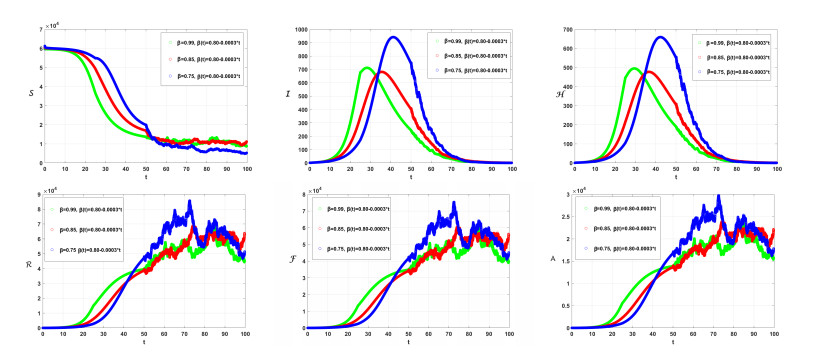
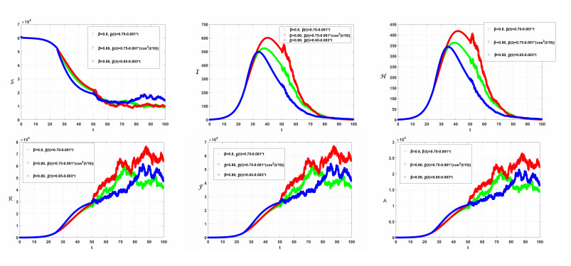
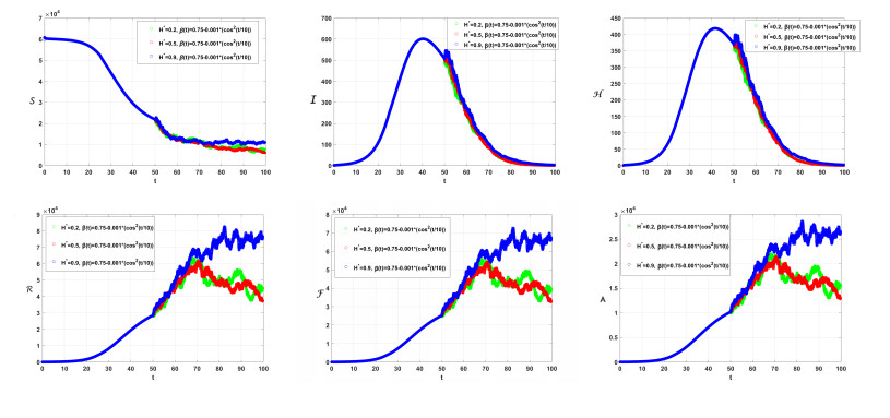
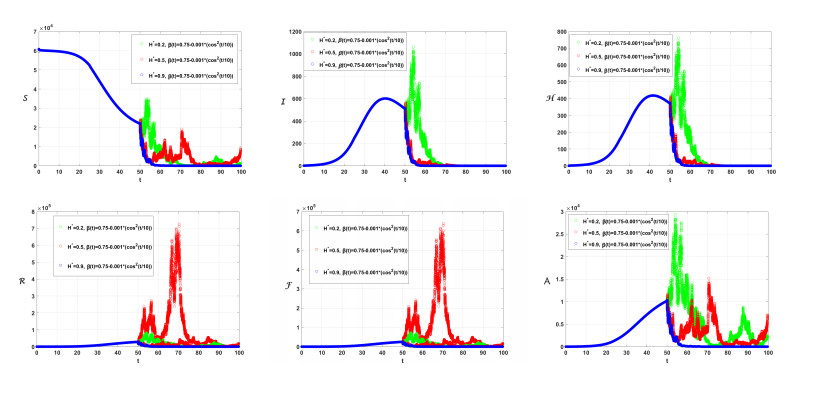
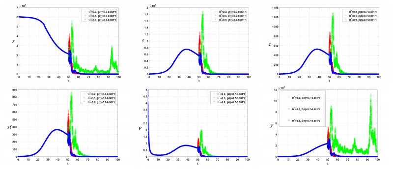
To obtain the numerical solutions for the proposed piecewise models (2.9)–(2.14), we employ the following parameters: $a = 6.82621 10^{-5},$ $b = 1.0648 10^{-4},$ $c = 2.0478 10^{-4},$ $d = 0.25,$ $f = 3.5,$ $g = 2.5 10^{-4},$ $\lambda = 2.21,$ $\mu = 0.10475,$ $v = 0.94,$ $u = 0.3$. The initial conditions are set as follows: $\mathcal{S}(0) = 59659,$ $\mathcal{I}(0) = 1,$ $\mathcal{E}(0) = 0,$ $\mathcal{P}(0) = 5,$ $\mathcal{A}(0) = 0,$ $\mathcal{R}(0) = 0,$ $\mathcal{H}(0) = 0,$ $\mathcal{R}(0) = 0,$ $\mathcal{F}(0) = 0,$ and $T_{1} = 25, T_{2} = 50,$ and $T_{f} = 100,$ $\Theta(\Delta \tau) = 1-e^{-\Delta \tau}$. The numerical results for (2.9)-(2.13) are graphically represented at various values of \(\beta \), \(\beta(\tau) \), \(\sigma_{i} \) (where \(i \) ranges from 1 to 8), and \(H^{\ast}(\tau) \). The simulations are conducted using the nonstandard Euler-Maruyama method (NEMM) (2.27) and the Caputo proportional constant-Grünwald-Letnikov nonstandard finite difference method CPC-GLNFDM (2.26). The dynamical behavior of the systems given by (2.9)–(2.13) is illustrated in Figures 1 through 5. It is observed that the crossover behavior is prominent around the values \(T_{1} = 25 \), \(T_{2} = 50 \), and \(T_{f} = 100 \). After these points, the dynamics exhibit multiplicity in their behavior. Figure 1 illustrates the simulation for (2.9)–(2.13) with $\beta(\tau) = 0.80-0.003t$ and $H^{\ast} = 0.7$, considering various values of $\beta$ and $\sigma_{i}$. Figure 2 demonstrates how the solutions behave under various scenarios, with different values of $\beta (\tau)$ and for $\beta = 0.8$, and $H^{\ast} = 0.7$. Figure 3 illustrates the change in the behavior of the solutions (2.9)–(2.13) when employing different values of $H^{\ast},$ $\beta(\tau) = 0.75-0.001(cos^2(\tau/10))$, and $\beta = 0.80, \sigma_{i} = 0.05$. Figure 4 illustrates the behavior of the solution of (2.9)–(2.13) for different values of $H^{\ast}$ and $\sigma_{i}$ $\beta(\tau) = 0.75-0.001(cos^2(\tau/10))$ and $\beta = 0.80$. To illustrate how parameter values $\sigma_{i}$ and $\mathcal{H}$ influence the results, we refer to Figure 5. From the simulation, we discerned several nuanced insights of the model, which proved invaluable insights from both biological and mathematical perspectives.

4.   Conclusions

In conclusion, a new mathematical model of piecewise fractional and variable-order differential equations and the fractional stochastic derivative of the COVID-19 epidemic has been developed. Moreover, two numerical techniques are constructed to solve the proposed model. These methods are the nonstandard modified Euler Maruyama method for the fractional stochastic model and the Caputo proportional constant-Grünwald-Letnikov nonstandard finite difference method for the fractional and variable-order deterministic models. Utilizing this approach has enriched our understanding of the dynamics underlying this intricate health crisis. Furthermore, by integrating fractional Brownian motion into stochastic differential equations, we have gleaned valuable insights into the unpredictable nature of infectious disease propagation. The development of two specialized numerical methods, namely, Caputo's proportional constant-Grünwald-Letnikov nonstandard finite difference method and the nonstandard modified Euler Maruyama technique, enabled us to delve deeply into the behavior of our extended models. Through a series of numerical tests, we have showcased the efficiency of these methods and garnered robust empirical support for our theoretical findings. Perhaps most crucially, our research has paved new pathways for studying the COVID-19 pandemic. The extended models afford the flexibility to examine a broad spectrum of behaviors, from deterministic patterns to stochastic processes. This allows for more adaptive strategies and interventions as circumstances change. This study stands as a substantial contribution to epidemiology, offering indispensable tools and insights that can guide public health decisions and aid in addressing the ongoing global health crisis.

Use of AI tools declaration

The authors declare they have not used Artificial Intelligence (AI) tools in the creation of this article.

Acknowledgments

The authors are thankful to the Deanship of Scientific Research at Najran University for funding this work under the Research Priorities and Najran Research funding program grant code (NU/NRP/SERC/12/3).

Conflicts of Interest:

The authors declare no conflicts of interest.

Appendix.   Proofs of Lemmas 2.1 and 2.2

Proof of Lemma 2.1. Let $X \in \bar{B}(X_0, \varDelta)$, then

where

and this complete the proof. □

Proof of Lemma 2.2. Let $X = (\mathcal{S}, \mathcal{E}, \mathcal{I}, \mathcal{P}, \mathcal{A}, \mathcal{H}, \mathcal{R}, \mathcal{F})$, $\bar{X} = (\bar{\mathcal{S}}, \bar{\mathcal{E}}, \bar{\mathcal{I}}, \bar{\mathcal{P}}, \bar{\mathcal{A}}, \bar{\mathcal{H}}, \bar{\mathcal{R}}, \bar{\mathcal{F}})\in \bar{B}(X_0, \varDelta)$ and we have

Also, we have for all $\wp_{1}, \, \wp_{2}, \, \upsilon_{1}, \, \upsilon_{2} \in \mathbb{R}$

and combining that with Lemma 2.1 we find

Also, we have

The linearity of the operators $\mathfrak{F}_{3}, \, \mathfrak{F}_{4}, \, \mathfrak{F}_{5}, \ \ \mathfrak{F}_{6}, \, \mathfrak{F}_{7}, \ \ \mathfrak{F}_{8}$

By rewriting the above equations in matrix form we find

where

□