I. Introduction

Research on digital currencies, especially cryptocurrencies, has increased tremendously, with exponential growth in recent years (Caporale et al., 2018). The novel coronavirus disease, or COVID-19, further piqued researchers’ interest as financial market variables responded negatively to the World Health Organization’s announcement of the pandemic in March 2020 (Salisu et al., 2020).

Several studies have tested whether cryptocurrencies are safe havens during the COVID-19 pandemic or diversifiers (see, for instance, Conlon et al., 2020; Corbet et al., 2020), sometimes juxtaposed with other assets such as gold and equities (see, for instance, González et al., 2021; Shehzad et al., 2021). The rationale for such studies emerged from the characteristics of cryptocurrencies, since these are decentralized and not controlled by any central bank or government, making them somewhat disconnected from the real economy (Caferra & Vidal-Tomás, 2021). Studies have found various results: cryptocurrencies can either be safe havens or not, perhaps because of the focus on different regions, as well as the different methodologies employed (Khelifa et al., 2021).

Only a few studies have examined the volatility and level of efficiency of cryptocurrencies before and during the COVID-19 pandemic. Yousaf & Ali (2020) note that the volatility of cryptocurrencies during the crisis period could cause portfolio managers and policymakers to diversify or mitigate risks by adjusting asset portfolios and policies, respectively. Yaya et al. (2021) also observe that a study of the efficiency of cryptocurrencies is useful for evaluating the investment environment, as well as developing the financial market. The authors based their conclusion on Fama’s (1970) hypothesis that market efficiency, and not domestic or macroeconomic policy, implies that only the past information of prices predicts their future.

Sarkodie et al. (2021) analyze the impact of the COVID-19 pandemic on the volatility of cryptocurrency prices using the novel Romano–Wolf multiple hypothesis testing method. They found that Litecoin prices surged by about 3.20–3.84%, Bitcoin by 2.71–3.27%, Ethereum by 1.43–1.75%, and Bitcoin Cash by 1.34–1.62% due to COVID-19 shocks. Similarly, Lahmiri & Bekiros (2020), using approximate entropy and largest Lyapunov exponents, find that cryptocurrencies became more volatile during the COVID-19 pandemic. Mnif et al. (2020) evaluate the level of efficiency of five cryptocurrencies using multifractal analysis prior to and after the COVID-19 outbreak. They found that the most efficient cryptocurrency before the outbreak was Bitcoin, but it became less efficient than Ethereum after the outbreak. However, all the cryptocurrencies they evaluated became more efficient after the start of the COVID-19 pandemic.

This paper differs from other studies because it assesses the announcement effect of the COVID-19 pandemic on the efficiency of cryptocurrencies. One critical problem it investigates is whether the dynamic behavior of cryptocurrencies is predictable and contradicts Fama’s (1970) efficient market hypothesis (EMH)^[1], which states that prices should follow a random walk. Fama (1970) also show differences between forms of efficiency. The condition under which the current values of financial assets include all historical financial information is the weak form of the EMH. Therefore, the hypothesis suggests that investing in these financial assets cannot yield abnormal returns. The semi-strong EMH posits that the prices of financial assets reflect all the information available on the market at any given time, including historical prices and other historical information (thus incorporating the weak form of the EMH), with prices changing rapidly and without bias to reflect any new public information released on the market. Finally, the strong form of the EMH posits that prices integrate all available information on the market, including previous financial data (weak form), new public information (semi-strong form), and private information (strong form). However, the 2008 financial crisis called into doubt the efficient market theory, and whether the EMT is defective and cannot withstand price discovery has sparked debate among financial institutions, economists, and academics.

Long-memory methods such as fractional integration can be used to explore the stochastic characteristics of cryptocurrencies. The advantage of the fractional integration method is that it allows for significantly richer dynamics than traditional models based on the I(0)/I(1) dichotomy. Traditional econometric methods used nonstationary unit root tests to establish the order of integration of the series. However, it is already well documented that traditional unit root testing approaches (e.g., Dickey & Fuller, 1979; Phillips & Perron, 1988) have limited power compared to fractional alternatives (Hassler & Wolters, 1994).

Contrary to other studies that combine myriad cryptocurrencies, this paper focuses on only two cryptocurrencies, Bitcoin and Ethereum, which are considered the top cryptocurrencies in terms of market capitalization (Khelifa et al., 2021) and popularity (Chen et al., 2020).

The remainder of the paper is organized as follows: Section II presents the methodological approach; the data and results are discussed in Section III, and Section IV draws our conclusion.

II. Methodology

We apply a fractional integration model where the number of differences required to make a time series stationary, I(0), can be in fractional form and might not assume an integer value. Therefore, the fractionally integrated model for a time series $x_{\text{t}} = 1,2,\ldots,T$ can be specified as follows:

$$\left(1 - L\right)^{d}x_{t} = \alpha + \gamma Trend + \varepsilon_{t},\tag{1}$$

where $d$ is any real value and represents the order of integration, L is the lag operator $Lx_{t} = x$, and $x_{t}$ is the logarithmic return of the cryptocurrency series integrated by order $d$ and represented by $x_{t} \approx Id$ and $\varepsilon_{t}\sim N 0,\sigma_{\varepsilon}^{2} .$^[2]

For all real $d$, premised on its binomial expansion, the polynomial $(1-L)^d$ in equation (1) can be presented as follows:

$$\begin{align}\left(1 - L\right)^{d} =& \sum_{j = 0}^{\infty}{\phi_{j}L^{j} =}\sum_{j = 0}^{\infty}{\left(\begin{matrix} d \\ j \\ \end{matrix}\right) (- 1)^{j}L^{j}} \\&=1 - \text{dL} + \frac{d(d - 1)}{2}L^{2} - \ldots.\end{align}\tag{2}$$

Therefore,

$$(1 - L)^{d}\pi_{t} = x_{t} - dx_{t - 1} + \frac{d(d - 1)}{2}x_{t - 2} - \ldots \tag{3}.$$

Hence, equation (1) can be presented as

$$\begin{align} x_{t} =&\ \alpha + \gamma Trend + dx_{t - 1} + \frac{d(d - 1)}{2}Z_{t - 2} - \ldots . \\ &+ \varepsilon_{t}\end{align}\tag{4}$$

Equation (4) highlights the important role $d$ also plays in the calculation of the level of persistence in the cryptocurrencies series, since it describes the degree of dependence (long memory behavior) of the cryptocurrency series. Consequently, the higher the value of $d$, the higher will be the level of dependence between observations in the series and, consequently, the higher the degree of persistence. We assume the errors to be uncorrelated (white noise) and consider two different specifications of the model: (i) with an intercept and (ii) with a linear time trend.

Fama’s (1970) EMH postulates that, if markets are efficient, nothing except for past information about an asset predicts the future dynamics of market prices; macroeconomic policy and other factors do not impact prices. Consequently, returns would be unpredictable in an efficient market (random walk hypothesis), whereas, in an inefficient market, they would be predictable, leading to investors making abnormal returns.

Three results are possible depending on the value of $d$. First, if $d=0$, then $x_t$ displays low-
level persistence (i.e., a short memory), and autocorrelations decay in an exponentially fast
manner, with the series being termed I(0), or covariance stationary, validating the EMH. Second,
if $d$ falls within the range of (0,0.5), then $x_{t}$ is termed as having long memory, due to the high degree of association between observations that are distant in time. However, this process is stationary and mean reverting. A fractional order between zero and one can still be used to validate the EMH if it is less than 0.5. Third, if $d \geq 0.5,$ then $x_{t}$ is presumed to be nonstationary but mean reverting, and the EMH does not hold. In the long memory scenario, $x_{t}$ can exhibit the properties of mean-reverting or non–mean-reverting processes based on the value of $d$. If $0.5 < d < 1$, then $x_{t}$ is mean reverting, and any policy will have a temporary influence on the series. Finally, if $d \geq 1,$ then $x_{t}$ is non–mean reverting, and any policy shock on the series will have a permanent effect on the series.

In this paper, we use the semiparametric model of Shimotsu & Phillips (2005) and the two-step exact local Whittle estimation of Shimotsu (2010), which is widely used in the literature. Shimotsu’s (2010) exact local Whittle estimation is an extension of the model of Shimotsu & Phillips (2005), and it addresses a process involving a time trend but whose mean is unknown.^[3] In addition to using the full sample, we split our data set into subsamples for the periods before and during the COVID-19 pandemic, respectively.^[4]

III. Data and Results

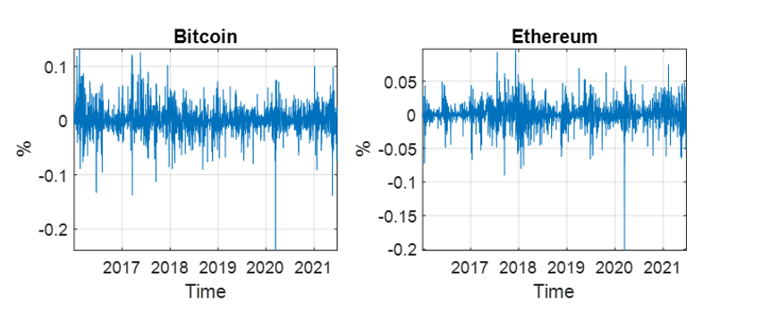
The dataset we use comprise the daily prices of the cryptocurrencies Bitcoin and Ethereum from January 2, 2016, to June 24, 2021. The log-transformed prices for the returns of Bitcoin and Ethereum are shown in Figure 1.

Figure 1.A time-series plot of returns for Bitcoin and Ethereum

Notes: This figure plots time series data for Bitcoin and Ethereum price returns. Returns are computed as $logx_{t} - logx_{t - 1}*100.$

Table 1 presents the results of our estimation. We start by estimating the difference parameter for the whole sample and the subsamples for the periods after COVID-19 had been declared a pandemic and before, respectively. The results show the presence of long memory in the data, since estimations of the long memory parameter d fall within the range (0, 0.5), validating the EMH in the cryptocurrency market.^[5] However, how persistence rose during the period after COVID-19 had been declared a pandemic is of particular interest. This finding appears to imply that the effect of announcing COVID-19 as pandemic impacted the series’ degree of persistence. Additionally, the fact that the difference parameter $d$ is less than one indicated some degree of mean reversion, with the impact of the shock taking a long time to dissipate.

IV. Conclusion

Using a fractional integration approach, this article examines the efficiency of cryptocurrency markets. Bitcoin and Ethereum were chosen as representative cryptocurrencies, since they are the top cryptocurrencies in terms of market capitalization. To evaluate market efficiency, we expect randomness in cryptocurrency returns. The fractional integrated parameter $d$ should therefore differ nonsignificantly from zero. We observe evidence of long memory in both subsamples tested, supporting the EMH. Additionally, we observe an increase in the degree of persistence after COVID-19 was announced as a pandemic, compared to before. This result tends to suggest that the introduction of COVID-19 altered the series’ degree of integration, despite the market still being efficient.

This empirical research could assist traders, portfolio managers, investors, and policymakers make better choices and implement strategies, since it demonstrates that cryptocurrency markets cannot be manipulated to generate extraordinary gains. Further research is needed to update these results as the COVID-19 epidemic unfolds.